Chapter 5 Data-cubes or SpatRaster
Whats is a Spatraster?
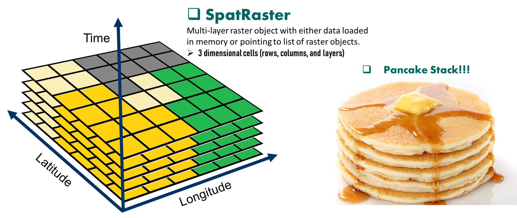
In addition, a SpatRaster can store information about the file in which the raster cell values are stored (equivalent to Raster Stack). Or, if there is no such file, a SpatRaster can hold the cell values in memory (equivalent to Raster Brick from the older raster package).
Note: Raster operations on cell values stored in memory are usually faster but computationally intensive.
5.1 Create, subset and visualize SpatRaster
We will create multilayer SpatRaster for NDVI and SMAP SM from the sample dataset and demonstrate several applications and operations. Working with SpatRaster is very similar to working with regular arrays or lists.
###############################################################
#~~~ Create and plot NDVI SpatRaster
library(terra)

# Location of the NDVI raster files
ndvi_path="./SampleData-master/raster_files/NDVI/" #Specify location of NDVI rasters

# List of all NDVI rasters
ras_path=list.files(ndvi_path,pattern='*.tif',full.names=TRUE)
head(ras_path)
## [1] "./SampleData-master/raster_files/NDVI/NDVI_resamp_2016-01-01.tif"
## [2] "./SampleData-master/raster_files/NDVI/NDVI_resamp_2016-01-17.tif"
## [3] "./SampleData-master/raster_files/NDVI/NDVI_resamp_2016-02-02.tif"
## [4] "./SampleData-master/raster_files/NDVI/NDVI_resamp_2016-02-18.tif"
## [5] "./SampleData-master/raster_files/NDVI/NDVI_resamp_2016-03-05.tif"
## [6] "./SampleData-master/raster_files/NDVI/NDVI_resamp_2016-03-21.tif"Let’s import NDVI rasters from the location and store as a 3D data cube. We will use lapply, map, and for loop using addlayer function to import rasters from paths stored ras_list. We will also learn how to add shapefiles to the background of all plots made using RasterBrick/Stack.
# Method 1: Use lapply to create raster layer list from the raster location
ras_list = lapply(paste(ras_path, sep = ""), rast)
#This a list of 23 raster objects stored as individual elements.

#Convert raster layer lists to data cube/Spatraster
ras_stack = rast(ras_list)     # Stacking all rasters as a data cube!!!
# This a multi-layer (23 layers in this case) SpatRaster Object.

#inMemory() reports whether the raster data is stored in memory or on disk.
inMemory(ras_stack[[1]])
## [1] FALSE# Method 2: Using pipes to create raster layers from the raster location
library(tidyr) # For piping
ras_list = ras_path %>% purrr::map(~ rast(.x)) # Import the raster
ras_stack = rast(ras_list) # Convert RasterStack to RasterBrick
# Method 3: Using for loop to create raster layers from the raster location
ras_stack=rast()
for (nRun in 1:length(ras_path)){
ras_stack=c(ras_stack,rast(ras_path[[nRun]]))
}
# Check dimension of data cube
dim(ras_stack) #[x: y: z]- 23 raster layers with 456 x 964 cells## [1] 456 964 23## [1] 23## [1] "NDVI_resamp_2016-01-01" "NDVI_resamp_2016-01-17" "NDVI_resamp_2016-02-02"
## [4] "NDVI_resamp_2016-02-18" "NDVI_resamp_2016-03-05" "NDVI_resamp_2016-03-21"
## [7] "NDVI_resamp_2016-04-06" "NDVI_resamp_2016-04-22" "NDVI_resamp_2016-05-08"
## [10] "NDVI_resamp_2016-05-24" "NDVI_resamp_2016-06-09" "NDVI_resamp_2016-06-25"
## [13] "NDVI_resamp_2016-07-11" "NDVI_resamp_2016-07-27" "NDVI_resamp_2016-08-12"
## [16] "NDVI_resamp_2016-08-28" "NDVI_resamp_2016-09-13" "NDVI_resamp_2016-09-29"
## [19] "NDVI_resamp_2016-10-15" "NDVI_resamp_2016-10-31" "NDVI_resamp_2016-11-16"
## [22] "NDVI_resamp_2016-12-02" "NDVI_resamp_2016-12-18"# Subset raster stack/brick (notice the double [[]] bracket and similarity to lists)
sub_ras_stack=ras_stack[[c(1,3,5,10,12)]] #Select 1st, 3rd, 5th, 10th and 12th layers
#Try subsetting with dates:
Season<-str_subset(string = names(ras_stack), pattern = c("20..-0[3/4/5]"))
ras_stack[[Season]]## class : SpatRaster
## dimensions : 456, 964, 6 (nrow, ncol, nlyr)
## resolution : 0.373444, 0.373444 (x, y)
## extent : -180, 180, -85.24595, 85.0445 (xmin, xmax, ymin, ymax)
## coord. ref. : lon/lat WGS 84 (EPSG:4326)
## sources : NDVI_resamp_2016-03-05.tif
## NDVI_resamp_2016-03-21.tif
## NDVI_resamp_2016-04-06.tif
## ... and 3 more sources
## names : NDVI_~03-05, NDVI_~03-21, NDVI_~04-06, NDVI_~04-22, NDVI_~05-08, NDVI_~05-24
## min values : -0.2000000, -0.175517, -0.1699783, -0.1848017, -0.199075, -0.1863334
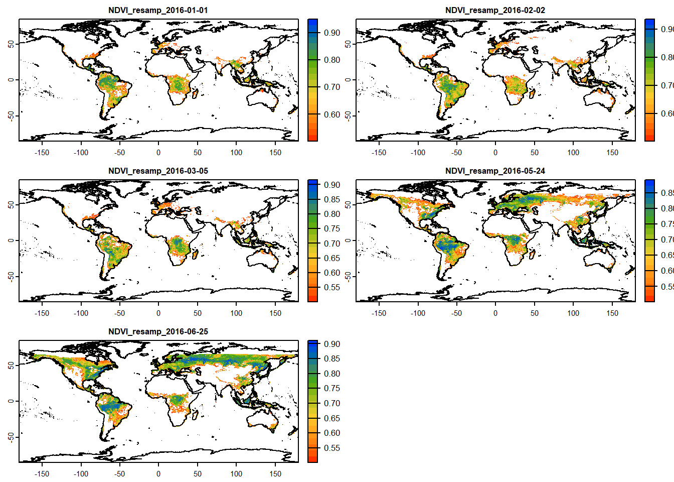
## max values : 0.9168695, 0.909500, 0.9042087, 0.9123000, 0.944600, 0.8917526#~~ Plot first 4 elements of NDVI SpatRaster
# Function to add shapefile to a raster plot
addCoastlines=function(){
plot(vect(coastlines), add=TRUE) #convert 'coastlines' to vector format
}
terra::plot(sub_ras_stack[[1:4]], # Select raster layers to plot
col=mypal2, # Specify colormap
asp=NA, # Aspect ratio= NA
fun=addCoastlines) # Add coastline to each layer
Expert Note: For memory intensive rasters to brick formation, the “for” loop method may be better to avoid memory bottleneck.
5.2 Geospatial operations on SpatRaster
In this section, we will demonstrate application of several operations on SpatRaster for e.g. extracting time series at user-defined locations, spatial data extraction using spatial polygons/raster, crop and masking of SpatRaster.
5.2.1 Time-series extraction from SpatRaster
Raster extraction is the process of identifying and returning the values associated with a ‘target’ raster at specific locations, based on a vector object. The results depend on the type of vector object used (points, lines or polygons) and arguments passed to the terra::extract() function.
We will demonstrate two ways of extracting time series information from SpatRaster.
Method 1: Using terra::extract function to extract time series data for specific location(s)
###############################################################
#~~~~ Method 1.1: Extract values for a single location

# User defined lat and long
Long=-96.33; Lat=30.62
# Creating a spatial vector object from the location coords
college_station = vect(SpatialPoints(cbind(Long, Lat)))


# Extract time series for the location
ndvi_val=terra::extract(ras_stack,
                 college_station,    # lat-long as spatial locations
                 method='bilinear')  # or "simple" for nearest neighbor

# Create a dataframe using the dates (derived from raster layer names) and extracted values
ndvi_ts=data.frame(Time=c(1:nlyr(ras_stack)), # Sequence of retrieval time
                   NDVI=as.numeric(ndvi_val[,-1]))     #NDVI values
# Try changing Time to as.Date(substr(colnames(ndvi_val),13,22), format = "%Y.%m.%d")

# Plot NDVI time series extracted from raster brick/stack
plot(ndvi_ts, type="l", col="maroon", ylim=c(0.2,0.8))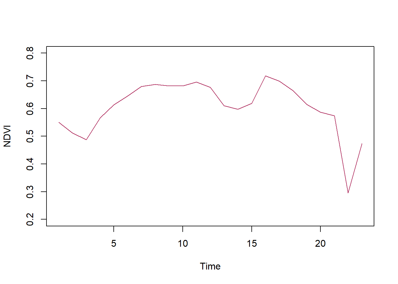
Let us now extract values for multiple locations.
#~~~~ Method 1.2:  Extract values for multiple locations
# Import sample locations from contrasting hydroclimate
library(readxl)
loc= read_excel("./SampleData-master/location_points.xlsx")
print(loc)
## # A tibble: 3 × 4
## Aridity State Longitude Latitude
## <chr> <chr> <dbl> <dbl>
## 1 Humid Louisiana -92.7 34.3
## 2 Arid Nevada -116. 38.7
## 3 Semi-arid Kansas -99.8 38.8# Extract time series using "raster::extract"
loc_ndvi=terra::extract(ras_stack,
#2-column matrix or data.frame with lat-long
loc[,3:4],
# Use bilinear interpolation (or simple) option
method='bilinear')The rows in loc_ndvi variable corresponds to the points specified by the user, namely humid, arid and semi-arid locations. Let’s plot the extracted NDVI for three locations to look for patterns (influence on climate on vegetation).
# Create a new data frame with dates of retrieval and NDVI for different hydroclimates
library(lubridate)
ndvi_locs = data.frame(Date=ymd(substr(colnames(ndvi_val[,-1]),13,22)),
                      Humid = as.numeric(loc_ndvi[1,-1]),    #Location 1
                      Arid = as.numeric(loc_ndvi[2,-1]),     #Location 2
                      SemiArid = as.numeric(loc_ndvi[3,-1])) #Location 3

# Convert data frame in "long" format for plotting using ggplot
library(tidyr)
df_long=ndvi_locs %>% gather(Climate,NDVI,-Date)
#"-" sign indicates decreasing order
head(df_long,n=4)
## Date Climate NDVI
## 1 2016-01-01 Humid 0.5919486
## 2 2016-01-17 Humid 0.5762772
## 3 2016-02-02 Humid 0.5570874
## 4 2016-02-18 Humid 0.5752835# Plot NDVI for different locations (hydroclimates). Do we see any pattern??
library(ggplot2)
l = ggplot(df_long, # Dataframe with input Dataset
aes(x=Date, # X-variable
y=NDVI, # Y-variable
group=Climate)) + # Group by climate
geom_line(aes(color=Climate))+ # Line color based on climate variable
geom_point(aes(color=Climate))+ # Point color based on climate variable
theme_classic()
print(l)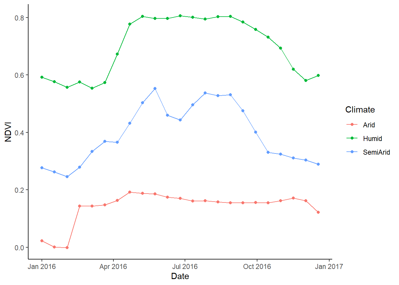
Method 2: Use rowFromY or rowFromX to find row and column number of the raster for the location.
###############################################################
#~~~~ Method 2: Retrieve values using cell row and column number
row = rowFromY(ras_stack[[1]], Lat)    # Gives row number for the selected Lat
col = colFromX(ras_stack[[1]], Long)   # Gives column number for the selected Long
ras_stack[row,col][1:5]                # First five elements of data cube for selected x-y
## NDVI_resamp_2016-01-01 NDVI_resamp_2016-01-17 NDVI_resamp_2016-02-02
## 1 0.5614925 0.5193725 0.4958409
## NDVI_resamp_2016-02-18 NDVI_resamp_2016-03-05
## 1 0.5731566 0.62595345.2.2 Spatial extraction/summary from SpatRaster
Let’s try extracting values of SpatRaster (for all layers simultaneously) based on polygon features using extract function.
#~~~~ Method 1: Extract values based on spatial polygons
IPCC_shp = read_sf("./SampleData-master/CMIP_land/CMIP_land.shp")

# Calculates the 'mean' of all cells within each feature of 'IPCC_shp' for each layers
ndvi_sp = terra::extract(ras_stack,   # Data cube
                         vect(IPCC_shp),    # Shapefile for feature reference
                         fun=mean,
                         na.rm=T,
                         #df=TRUE,
                         method='bilinear')

head(ndvi_sp,n=3)[1:5]
## ID NDVI_resamp_2016-01-01 NDVI_resamp_2016-01-17 NDVI_resamp_2016-02-02
## 1 1 -0.08325353 -3.320059e+38 -3.319744e+38
## 2 2 0.02765715 -2.329463e+38 -2.328498e+38
## 3 3 0.21922899 -1.435967e+37 -1.435967e+37
## NDVI_resamp_2016-02-18
## 1 -3.319115e+38
## 2 -2.330106e+38
## 3 -1.435967e+37We can also use a classified raster like aridity data we previously used, to extract values corresponding to each class of values using lapply and selective filtering.
Note: The two rasters must have same extent and resolution.
#~~~~ Method 2: Extract values based on another raster
aridity = rast("./SampleData-master/raster_files/aridity_36km.tif")

# Create an empty list to store extracted feature
climate_ndvi = list()
# Extracts the time series of NDVI for pixels for each climate region
climate_ndvi = lapply(list(1,2,3,4,5),function(x) (na.omit((ras_stack[aridity==x]))))

# Calculate and store mean NDVI for each climate region
climate_ndvi_mean = lapply(list(1,2,3,4,5),function(x) (mean(ras_stack[aridity==x], na.rm=TRUE)))

plot(unlist(climate_ndvi_mean),
     type = "b",
     ylab = "Climate_NDVI_Mean",
     xlab = "Aridity Index")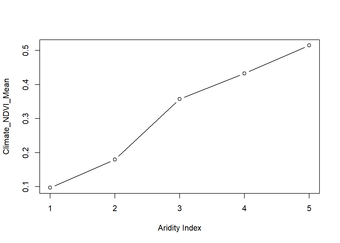
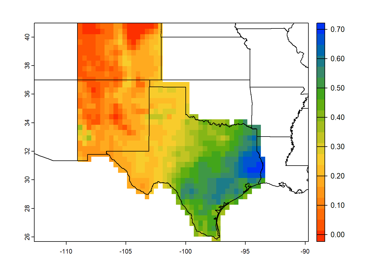
5.2.3 Crop and mask SpatRaster
We will now crop and mask SpatRaster using shapefile from the disk or from imported shapefile from spData::us_states. crop function clips the raster to the extent provided. mask removes the area outside the provided shapefile. Alternatively, we can import shapefile from disk using read_sf function.
# Import polygons for polygons for USA at level 1 i.e. state from disk

state_shapefile = read_sf("./SampleData-master/USA_states/cb_2018_us_state_5m.shp")

# Alternatively, use dataset from 'spData' package 'spData::us_states'

# Print variable names
names(state_shapefile)
## [1] "STATEFP" "STATENS" "AFFGEOID" "GEOID" "STUSPS" "NAME"
## [7] "LSAD" "ALAND" "AWATER" "geometry"## [1] "Nebraska"
## [2] "Washington"
## [3] "New Mexico"
## [4] "South Dakota"
## [5] "Texas"
## [6] "California"
## [7] "Kentucky"
## [8] "Ohio"
## [9] "Alabama"
## [10] "Georgia"
## [11] "Wisconsin"
## [12] "Oregon"
## [13] "Pennsylvania"
## [14] "Mississippi"
## [15] "Missouri"
## [16] "North Carolina"
## [17] "Oklahoma"
## [18] "West Virginia"
## [19] "New York"
## [20] "Indiana"
## [21] "Kansas"
## [22] "Idaho"
## [23] "Nevada"
## [24] "Vermont"
## [25] "Montana"
## [26] "Minnesota"
## [27] "North Dakota"
## [28] "Hawaii"
## [29] "Arizona"
## [30] "Delaware"
## [31] "Rhode Island"
## [32] "Colorado"
## [33] "Utah"
## [34] "Virginia"
## [35] "Wyoming"
## [36] "Louisiana"
## [37] "Michigan"
## [38] "Massachusetts"
## [39] "Florida"
## [40] "United States Virgin Islands"
## [41] "Connecticut"
## [42] "New Jersey"
## [43] "Maryland"
## [44] "South Carolina"
## [45] "Maine"
## [46] "New Hampshire"
## [47] "District of Columbia"
## [48] "Guam"
## [49] "Commonwealth of the Northern Mariana Islands"
## [50] "American Samoa"
## [51] "Iowa"
## [52] "Puerto Rico"
## [53] "Arkansas"
## [54] "Tennessee"
## [55] "Illinois"
## [56] "Alaska"# Exclude states outside of CONUS
conus = state_shapefile[!(state_shapefile$NAME %in% c("Alaska","Hawaii","American Samoa",
"United States Virgin Islands","Guam", "Puerto Rico",
"Commonwealth of the Northern Mariana Islands")),]
# plot CONUS as a vector using terra package
terra::plot(vect(conus)) 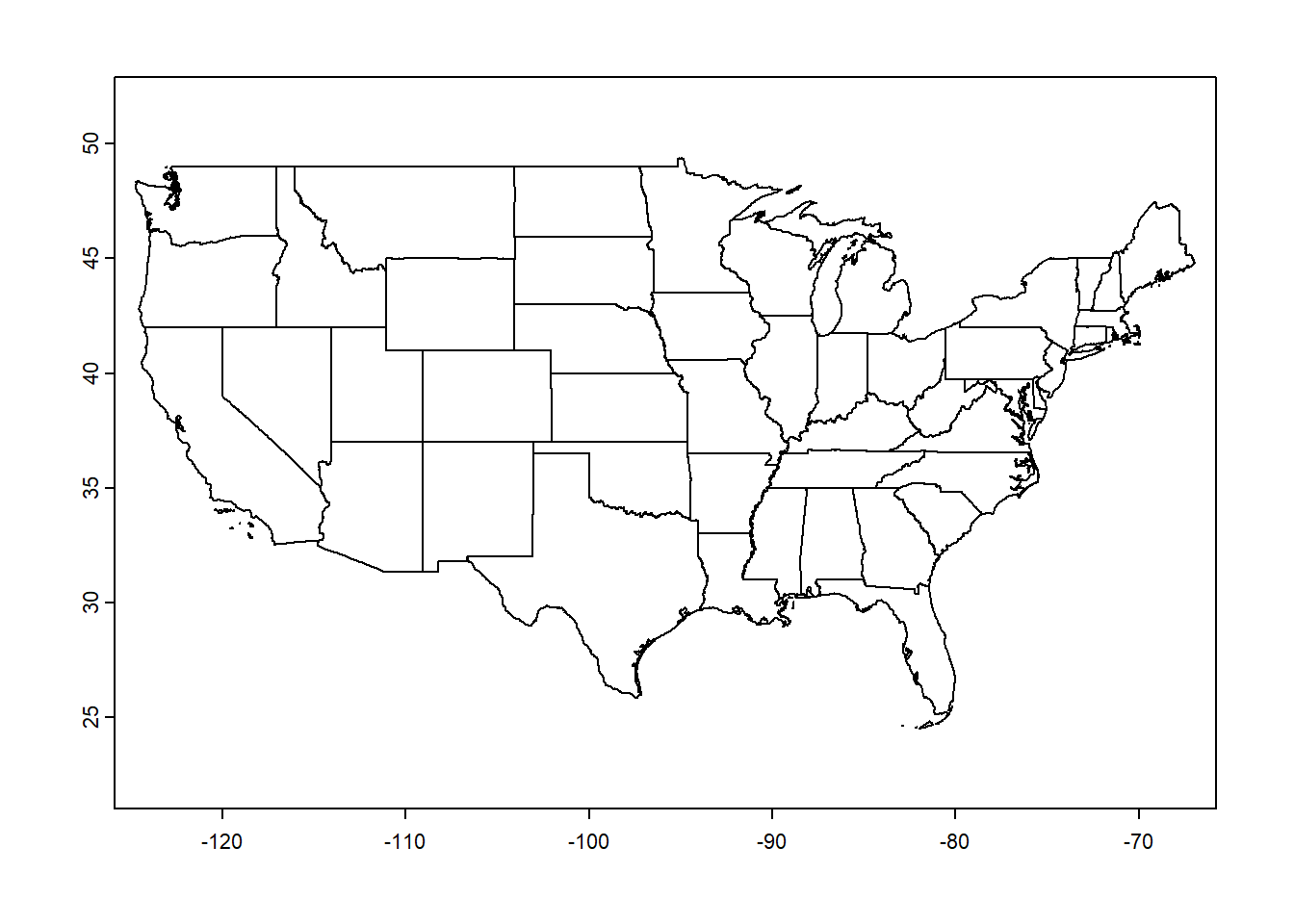
# Crop SpatRaster using USA polygon
usa_crop = crop(ras_stack, ext(conus))       # Crop raster to CONUS extent

# Plot cropped raster
plot(usa_crop[[1:4]], col=mypal2)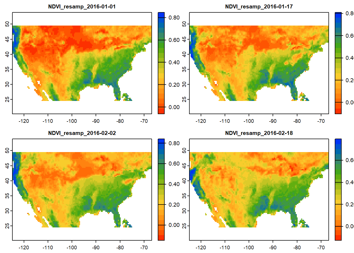
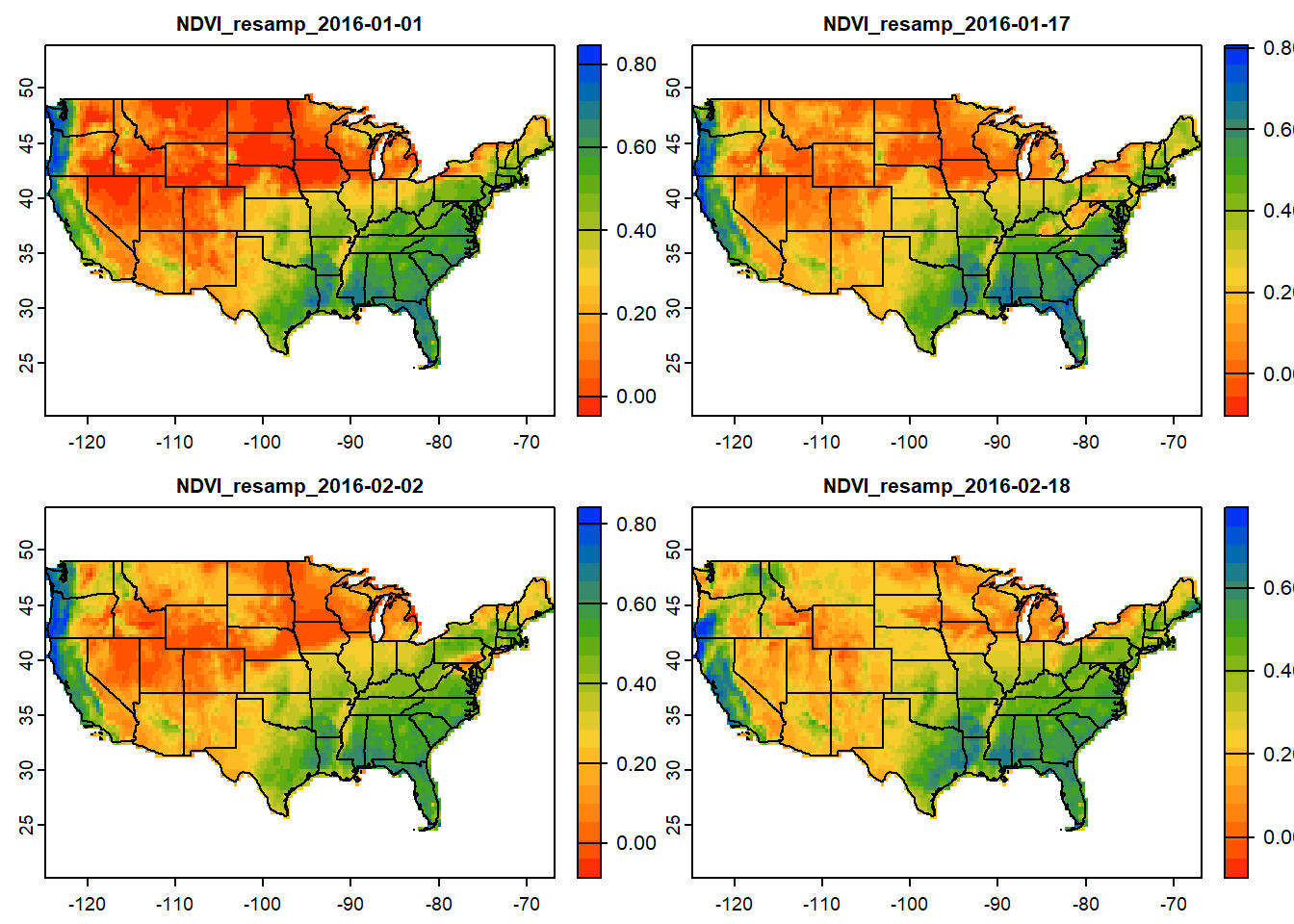
# Mask SpatRaster using USA polygon
ndvi_mask_usa = terra::mask(usa_crop, vect(conus))    # Mask raster to CONUS

# Mask SpatRaster using USA polygon
plot(ndvi_mask_usa[[1:4]],
     col=mypal2,
     fun=function(){plot(vect(conus), add=TRUE)} # Add background states
)
Let’s crop raster for selected US states.
# Mask raster for selected states
states = c('Colorado','Texas','New Mexico')

# Subset the selected states from CONUS shapefile
state_plot = state_shapefile[(state_shapefile$NAME %in% states),]

# Raster operation
states_trim = crop(ras_stack, ext(state_plot))                # Crop raster
ndvi_mask_states = terra::mask(states_trim, vect(state_plot)) # Mask

# Plot raster and shapefile
plot(ndvi_mask_states[[1]],
     col=mypal2,
     fun=function(){plot(vect(conus), add=TRUE)} # Add background states
     )
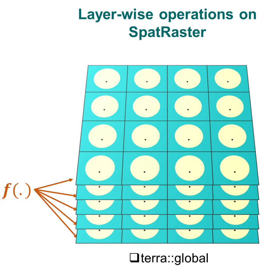
5.3 Layer-wise operations on SpatRaster
We will demonstrate common layer-wise arithmetic operations, summary statistics and data transformation on SpatRaster.
Arithmetic operations a.k.a arith-generic (+, -, *, /, ^, %%, %/%) on SpatRaster closely resemble simple vector-like operations. More details on arith-generic can be found here: https://rdrr.io/cran/terra/man/arith-generic.html.
For layer-wise summary statistics and user-defined operations, we will use global function.
Let’s try some layer-wise cell-statistics:
###############################################################
#~~~ Layer-wise cell-statistics
# Layer-wise Mean
global(sub_ras_stack, mean, na.rm= T) # Mean of each raster layer. Try modal, median, min etc.
## mean
## NDVI_resamp_2016-01-01 0.2840846
## NDVI_resamp_2016-02-02 0.2948298
## NDVI_resamp_2016-03-05 0.3057182
## NDVI_resamp_2016-05-24 0.4618550
## NDVI_resamp_2016-06-25 0.4997354## X25. X75.
## NDVI_resamp_2016-01-01 0.07188153 0.5135894
## NDVI_resamp_2016-02-02 0.08442930 0.5177374
## NDVI_resamp_2016-03-05 0.09917563 0.5113073
## NDVI_resamp_2016-05-24 0.23671686 0.6695234
## NDVI_resamp_2016-06-25 0.26000642 0.7303487# User-defined statistics by defining own function
quant_fun = function(x) {quantile(x, probs = c(0.25, 0.75), na.rm=TRUE)}
global(sub_ras_stack, quant_fun) # 25th, and 75th percentile of each layer## X25. X75.
## NDVI_resamp_2016-01-01 0.07188153 0.5135894
## NDVI_resamp_2016-02-02 0.08442930 0.5177374
## NDVI_resamp_2016-03-05 0.09917563 0.5113073
## NDVI_resamp_2016-05-24 0.23671686 0.6695234
## NDVI_resamp_2016-06-25 0.26000642 0.7303487# Custom function for mean, variance and skewness
my_fun = function(x){
meanVal=mean(x, na.rm=TRUE) # Mean
varVal=var(x, na.rm=TRUE) # Variance
skewVal=moments::skewness(x, na.rm=TRUE) # Skewness
output=c(meanVal,varVal,skewVal) # Combine all statistics
names(output)=c("Mean", "Var","Skew") # Rename output variables
return(output) # Return output
}
global(sub_ras_stack, my_fun) # Mean, Variance and skewness of each layer## Mean Var Skew
## NDVI_resamp_2016-01-01 0.2840846 0.07224034 0.5409973
## NDVI_resamp_2016-02-02 0.2948298 0.06677124 0.5075244
## NDVI_resamp_2016-03-05 0.3057182 0.06171894 0.5018285
## NDVI_resamp_2016-05-24 0.4618550 0.05944947 -0.2721941
## NDVI_resamp_2016-06-25 0.4997354 0.06587261 -0.3392214## NDVI_resamp_2016.01.01 NDVI_resamp_2016.02.02 NDVI_resamp_2016.03.05
## Min. :-0.17 Min. :-0.19 Min. :-0.16
## 1st Qu.: 0.07 1st Qu.: 0.08 1st Qu.: 0.10
## Median : 0.19 Median : 0.22 Median : 0.23
## Mean : 0.28 Mean : 0.29 Mean : 0.31
## 3rd Qu.: 0.51 3rd Qu.: 0.52 3rd Qu.: 0.51
## Max. : 0.92 Max. : 0.90 Max. : 0.90
## NA's :77736 NA's :77094 NA's :77106
## NDVI_resamp_2016.05.24 NDVI_resamp_2016.06.25
## Min. :-0.18 Min. :-0.19
## 1st Qu.: 0.24 1st Qu.: 0.26
## Median : 0.50 Median : 0.55
## Mean : 0.46 Mean : 0.50
## 3rd Qu.: 0.67 3rd Qu.: 0.73
## Max. : 0.89 Max. : 0.91
## NA's :77100 NA's :77091Global cell-statistics can be calculated by converting SpatRaster to a vector and then using regular statistics functions. We will use as.vector() to convert rasters to vector array before arithmetic operation.
###############################################################
#~~~ Global cell-statistics

# By vectorizing the SpatRaster and finding statistics
min_val=min(as.vector(sub_ras_stack), na.rm=T)
max_val=max(as.vector(sub_ras_stack), na.rm=T)
print(c(min_val,max_val))
## [1] -0.20000 0.95065# Another example of statistics of vectorized SpatRaster
quant=quantile(as.vector(sub_ras_stack), c(0.01,0.99), na.rm=TRUE) #1st and 99th percentiles
print(quant)## 1% 99%
## -0.05663428 0.84776928Layer-wise arithmetic operations on SpatRaster:
###############################################################
#~~~ Layer-wise operations on SpatRaster

# Arithmetic operations on SpatRaster are same as lists
add = sub_ras_stack+10                  # Add a number to raster layers
mult = sub_ras_stack*5                  # Multiply a number to raster layers
subset_mult = sub_ras_stack[[1:3]]*10   # Multiply a number to a subset of raster layers

# Data filtering based on cell-value
filter_stack = sub_ras_stack            # Create a RasterBrick to operate on
filter_stack[filter_stack<0.5] = NA     # Assign NA to any value less than 0.5

# Let's plot the filtered rasters
plot(filter_stack,
     col=mypal2,  # Color pal
     asp=NA,      # Aspect ratio: NA, fill to plot space
     nc=2,        # Number of columns to arrange plots
    fun=function(){plot(vect(coastlines), add=TRUE)} # Add background map
) 
# Layer-wise Log-transformation
log_ras_stack=log(sub_ras_stack)

# Normalize raster layers to [0,1] based on min and max of raster brick/stack
norm_stk=(sub_ras_stack-min_val)/(max_val-min_val) # Notice that the values are between [0,1]

# Plot in Robinson projection
mypal3 = cetcolor::cet_pal(20, name = "l5")
unikn::seecol(mypal3)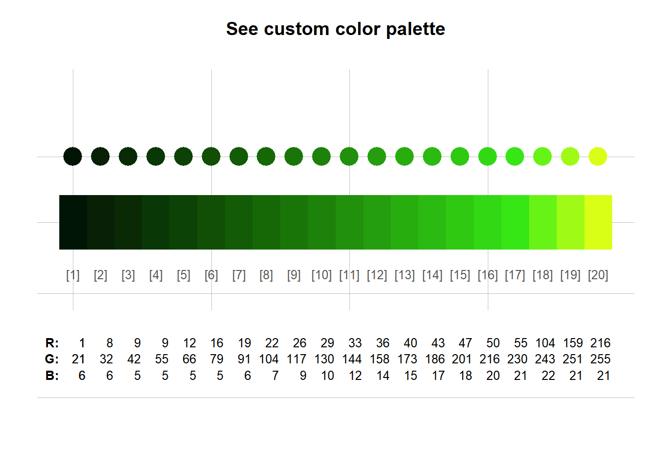
WorldSHP = st_as_sf(spData::world)
norm_NDVI= tm_shape(WorldSHP, projection = 'ESRI:54030',
ylim = c(-65, 90)*100000,
xlim = c(-152,152)*100000,
raster.warp = T)+
tm_sf()+
tm_shape(norm_stk[[2:5]], projection = 'ESRI:54030', raster.warp = FALSE) +
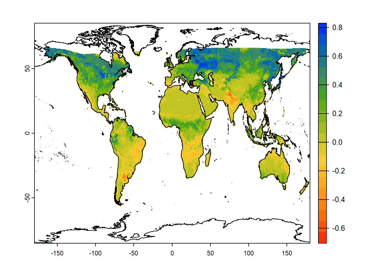
tm_raster(palette = rev(mypal3), title = "Normalized NDVI", style = "cont")+
tm_layout(main.title = "NDVI",
main.title.fontfamily = "Times",
legend.show = T,
legend.outside = T,
legend.outside.position = c("right", "top"),
frame = FALSE,
#earth.boundary = c(-160, -65, 160, 88),
earth.boundary.color = "grey",
earth.boundary.lwd = 2,
fontfamily = "Times")+
tm_graticules(alpha = 0.2, # Add lat-long graticules
labels.inside.frame = FALSE,
col = "lightgrey", n.x = 4, n.y = 3)+
tm_facets(ncol = 2)
print(norm_NDVI)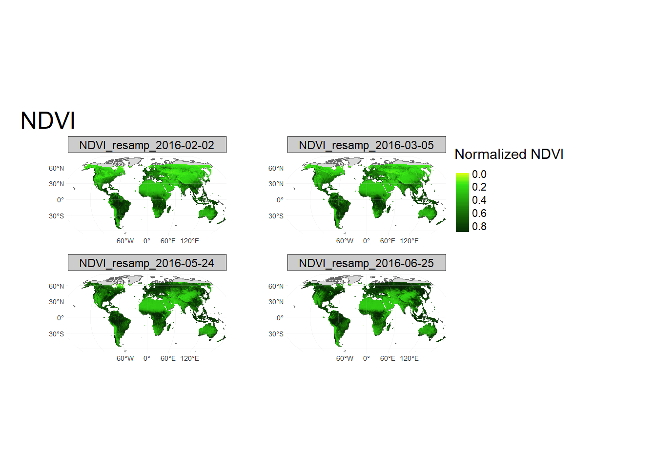
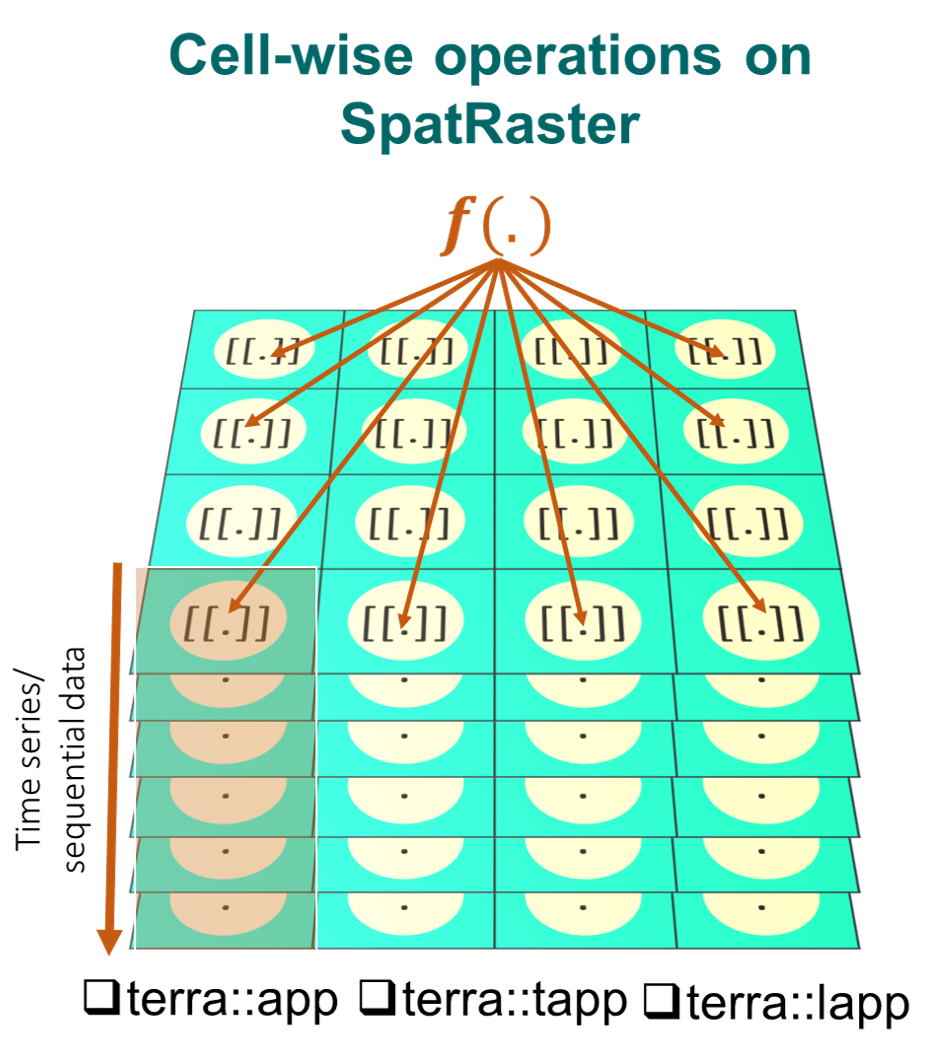
5.4 Cell-wise operations with app, lapp, tapp
We will now carry-out cell-wise operations on SpatRaster using the app(), tapp() and lapp() functions. These functions carry operations on each cell of a SpatRaster for all layers and are generally used to summarize the values of multiple layers into one layer. They are preferable in the presence of large raster datasets. Additionally, they allow you to save an output file directly.
5.4.1 app: Cell-wise operation on all layers
The app() function applies a function to each cell of a raster and is used to summarize (e.g., calculating the sum) the values of multiple layers into one layer.
#Let's look at the help section for app()
?terra::app
# Calculate mean of each grid cell across all layers
mean_ras = app(sub_ras_stack, fun=mean, na.rm = T)
# Calculate sum of each grid cell across all layers
sum_ras = app(sub_ras_stack, fun=sum, na.rm = T)
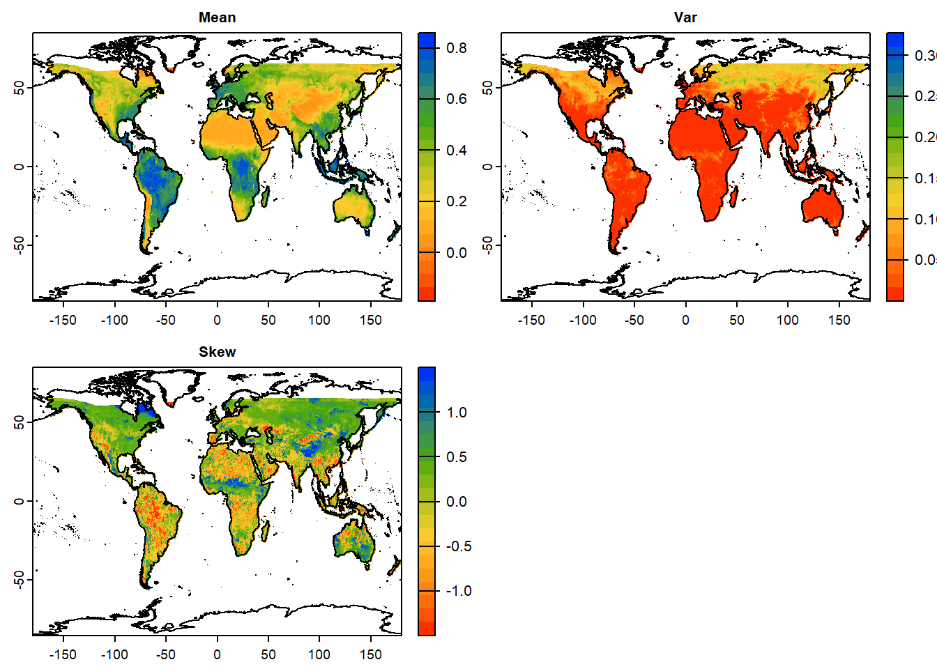
#~~ A user-defined function for mean, variance and skewness
my_fun = function(x){
meanVal=mean(x, na.rm=TRUE) # Mean
varVal=var(x, na.rm=TRUE) # Variance
skewVal=moments::skewness(x, na.rm=TRUE) # Skewness
output=c(meanVal,varVal,skewVal) # Combine all statistics
names(output)=c("Mean", "Var","Skew") # Rename output variables
return(output) # Return output
}
# Apply user function to each cell across all layers
stat_ras = app(sub_ras_stack, fun=my_fun)
# Plot statistics
plot(stat_ras,
col=mypal2, # Color pal
asp=NA, # Aspect ratio: NA, fill to plot space
nc=2, # Number of columns to arrange plots
fun=function(){plot(vect(coastlines), add=TRUE)} # Add background map
) DIY:Try plotting the same using
 tmap.
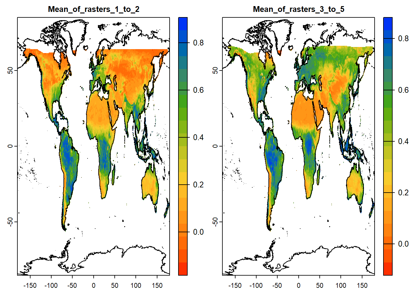
5.4.2 tapp: Cell-wise operation on layer groups
tapp() is an extension of app(), allowing us to select a subset of layers for which we want to perform a certain operation. Let’s have the first two layers as group 1 and the next three as group 2. Function will be applied to each group separately and 2 layers of output will be generated.
#Let's look at the help section for app()
?terra::tapp

#The layers are combined based on indexing.
stat_ras = terra::tapp(sub_ras_stack,
                     index=c(1,1,2,2,2),
                     fun= mean)

# Try other functions: "sum", "mean", "median", "modal", "which", "which.min", "which.max", "min", "max", "prod", "any", "all", "sd", "first".

names(stat_ras) = c("Mean_of_rasters_1_to_2", "Mean_of_rasters_3_to_5")
# Two layers are formed, one for each group of indices

# Lets plot the two output rasters
plot(stat_ras,
     col=mypal2,  # Color pal
     asp=NA,      # Aspect ratio: NA, fill to plot space
     nc=2,        # Number of columns to arrange plots
     fun=function(){plot(vect(coastlines), add=TRUE)} # Add background map
)
DIY: Try plotting the same using
 tidyterra.
5.4.3 lapp: layers as function arguments
The lapp() function allows to apply a function to each cell using layers as arguments.
#Let's look at the help section for app()
?terra::lapp

#User defined function for finding difference
diff_fun = function(a, b){ return(a-b) }

diff_rast = lapp(sub_ras_stack[[c(4, 2)]], fun = diff_fun)

#Plot NDVI difference
plot(diff_rast,
     col=mypal2,  # Color pal
     asp=NA,      # Aspect ratio: NA, fill to plot space
     nc=2,        # Number of columns to arrange plots
     fun=function(){plot(vect(coastlines), add=TRUE)} # Add background map
)