Chapter 4 Geospatial operations on raster/vector data
4.1 Raster resampling
We will demonstrate how to change the resolution of Spatraster files using terra::aggregate (fine to coarse), terra::disagg (coarse to fine), and resampling values from one raster to another using terra::resample function. We will use global aridity and soil moisture Spatrasters for this purpose.
In the newer terra package, the nearest‑neighbor resampling option has been renamed: instead of using method = “ngb” (as in the older raster package), you should now use method = “near”.
# Importing SMAP soil moisture data
sm=rast("./SampleData-master/raster_files/SMAP_SM.tif")

# Original resoluton of raster for reference
res(sm)
## [1] 0.373444 0.373444#~~ Aggregate raster to coarser resolution
SMcoarse = terra::aggregate(sm, # Soil moisture raster
fact = 10, # Aggregate by x 10
fun = mean) # Function used to aggregate values
res(SMcoarse)## [1] 3.73444 3.73444#~~ Disaggregate raster to finer resolution
SMfine = terra::disagg(sm,
fact=3,
method='bilinear')
res(SMfine)## [1] 0.1244813 0.1244813#~~ Raster resampling
# Import global aridity raster
aridity=rast("./SampleData-master/raster_files/aridity_36km.tif")
# Plot aridity map
terra::plot(aridity, col=mypal2, main= "Aridity Spatraster")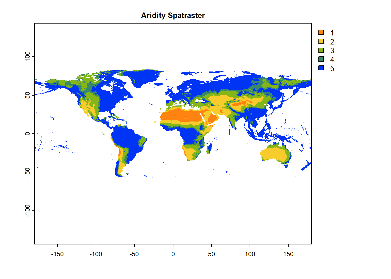
# Resample aridity raster to coarse resolution
aridityResamp=terra::resample(aridity,      # Original raster
                       SMcoarse,     # Target resolution raster
                       method='near') # bilinear or ngb (nearest neighbor)

# Plot resampled aridity map
terra::plot(aridityResamp, col=mypal2, main= "Aridity at Coarser Resolution")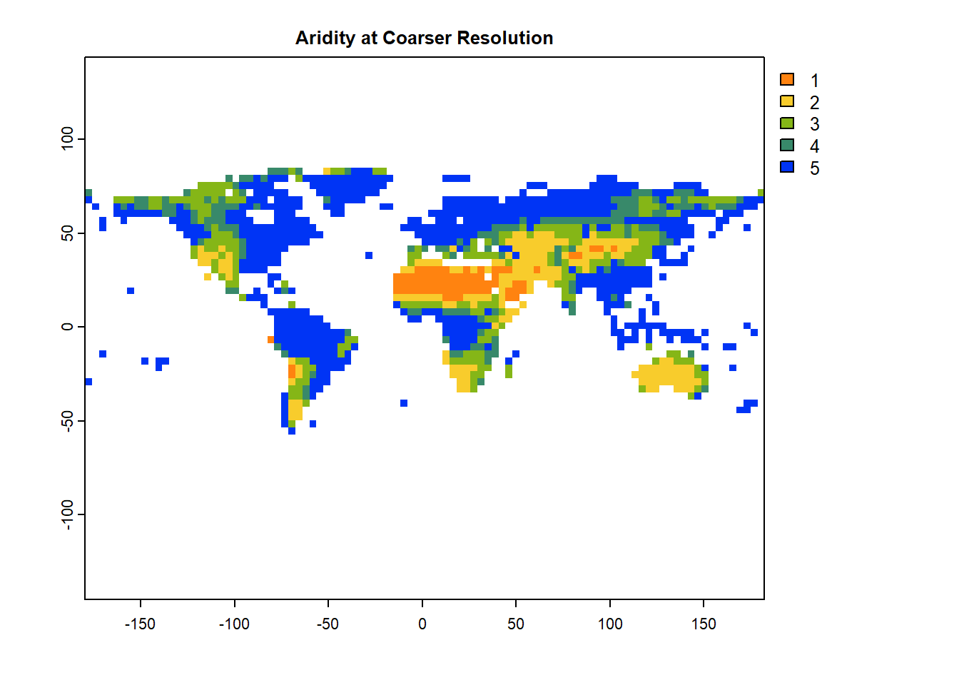
4.2 Raster summary statistics
Arithmetic operations a.k.a. arith-generic (+, -, *, /, ^, %%, %/%) on Spatrasters closely resemble simple vector-like operations. More details on arith-generic can be found here: https://rdrr.io/cran/terra/man/arith-generic.html.
We will use global function to apply summary statistics and user-defined operations on cells of a raster.
# Simple arithmetic operations
sm2=sm*2
print(sm2) # Try sm2=sm*10, or sm2=sm^2 and see the difference in sm2 values
## class : SpatRaster
## dimensions : 456, 964, 1 (nrow, ncol, nlyr)
## resolution : 0.373444, 0.373444 (x, y)
## extent : -180, 180, -85.24595, 85.0445 (xmin, xmax, ymin, ymax)
## coord. ref. : lon/lat WGS 84 (EPSG:4326)
## source(s) : memory
## varname : SMAP_SM
## name : SMAP_SM
## min value : 0.03999996
## max value : 1.75335217## mean
## SMAP_SM 0.209402## sd
## SMAP_SM 0.1434444## X25. X75.
## SMAP_SM 0.09521707 0.2922016# User-defined statistics by defining own function
quant_fun = function(x, na.rm=TRUE){ # Remember to add "na.rm" option
quantile(x, probs = c(0.25, 0.75), na.rm=TRUE)
}
global(sm, quant_fun) # 25th, and 75th percentile of each layer## X25. X75.
## SMAP_SM 0.09521707 0.2922016Note: With a multi-layered raster object, global will summarize each layer separately.
4.3 Summarizing rasters using shapefles
Let’s explore using a spatial polygon/shapefile for summarizing a raster (in this case, global SMAP soil moisture) by using extract function from the terra library. We will also transform global aridity raster to a polygon using as.polygons and st_as_sf functions to find the mean soil moisture values for each aridity class.
First, we will use the IPCC shapefile to summarize the soil moisture raster.
In the newer terra package, the extract() function no longer accepts the df=TRUE argument. That option was part of the older raster package. In terra, extract() already returns a data.frame (or SpatVector) by default, so specifying df=TRUE is unnecessary and will cause an error.
###############################################################
# Using shapefile to summarize a raster
sm_IPCC_df=terra::extract(sm,        # Spatraster to be summarized
                          vect(IPCC_shp),  # Shapefile/ polygon to summarize the raster
                          fun=mean,  # Desired statistic: mean, sum, min and max
                          na.rm=TRUE)# Ignore NA values? TRUE=yes!

head(sm_IPCC_df)
## ID SMAP_SM
## 1 1 0.2545766
## 2 2 0.3839087
## 3 3 0.2345457
## 4 4 0.3788003
## 5 5 0.2383580
## 6 6 0.1475145###############################################################
# Extract cell values for each region
sm_IPCC_list=terra::extract(sm, # Raster to be summarized
vect(IPCC_shp), # Shapefile/ polygon to summarize the raster
df=FALSE, # Returns a list
fun=NULL, # fun=NULL will output cell values within each region
na.rm=TRUE) # Ignore NA values? yes!
# Apply function on cell values for each region
library(tidyverse)
sm_IPCC_list %>%
as_tibble() %>%
group_by(ID) %>%
summarise(mean_SM = mean(SMAP_SM, na.rm =T))## # A tibble: 41 × 2
## ID mean_SM
## <dbl> <dbl>
## 1 1 0.255
## 2 2 0.384
## 3 3 0.235
## 4 4 0.379
## 5 5 0.238
## 6 6 0.148
## 7 7 0.110
## 8 8 0.336
## 9 9 0.399
## 10 10 0.320
## # ℹ 31 more rows#~~ Try user defined function
myfun=function (y){return(mean(y, na.rm=TRUE))} # User defined function for calculating means
sm_IPCC_list %>%
as_tibble() %>%
group_by(ID) %>%
summarise(mean_SM = myfun(SMAP_SM)) ## # A tibble: 41 × 2
## ID mean_SM
## <dbl> <dbl>
## 1 1 0.255
## 2 2 0.384
## 3 3 0.235
## 4 4 0.379
## 5 5 0.238
## 6 6 0.148
## 7 7 0.110
## 8 8 0.336
## 9 9 0.399
## 10 10 0.320
## # ℹ 31 more rows4.4 DIY: Summarize raster using classified raster
In the next example, we will convert global aridity raster into a polygon based on aridity classification using as.polygons and st_as_sf functions.
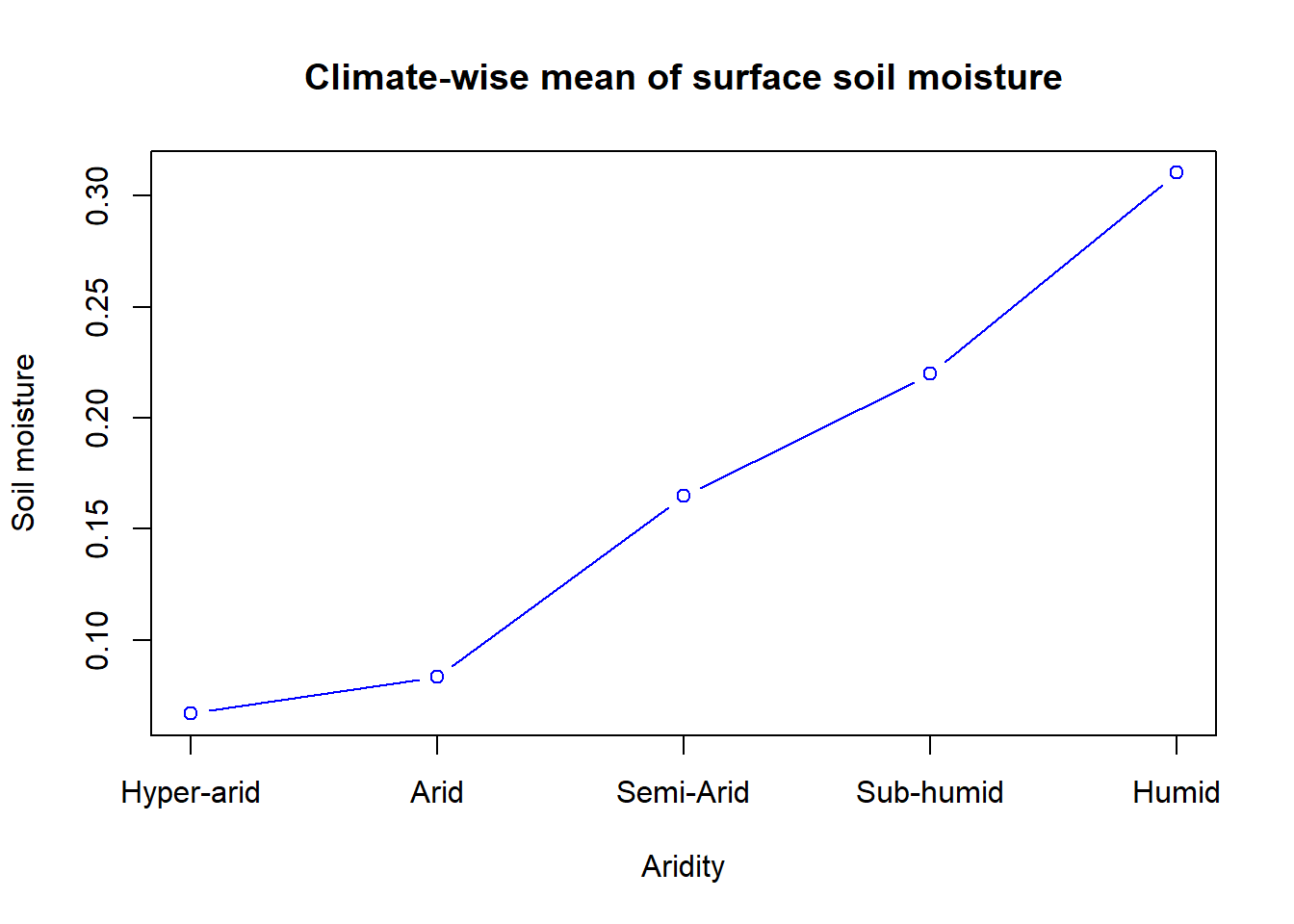
Global aridity raster has 5 classes with 5 indicating humid and 1 indicating hyper-arid climate. We will use this polygon to extract values from the Spatraster and summarize soil moisture for each aridity class.
###############################################################
#~~~ Convert a raster to a shapefile
aridity=rast("./SampleData-master/raster_files/aridity_36km.tif") #Global aridity

# Convert raster to shapefile
arid_poly=st_as_sf(as.polygons(aridity))   # Convert SpatRaster to polygon and then to sf

# Plot aridity polygon
terra::plot(arid_poly,
     col=arid_poly$aridity_36km)  # Colors based on aridity values (i.e. 1,2,3,4,5)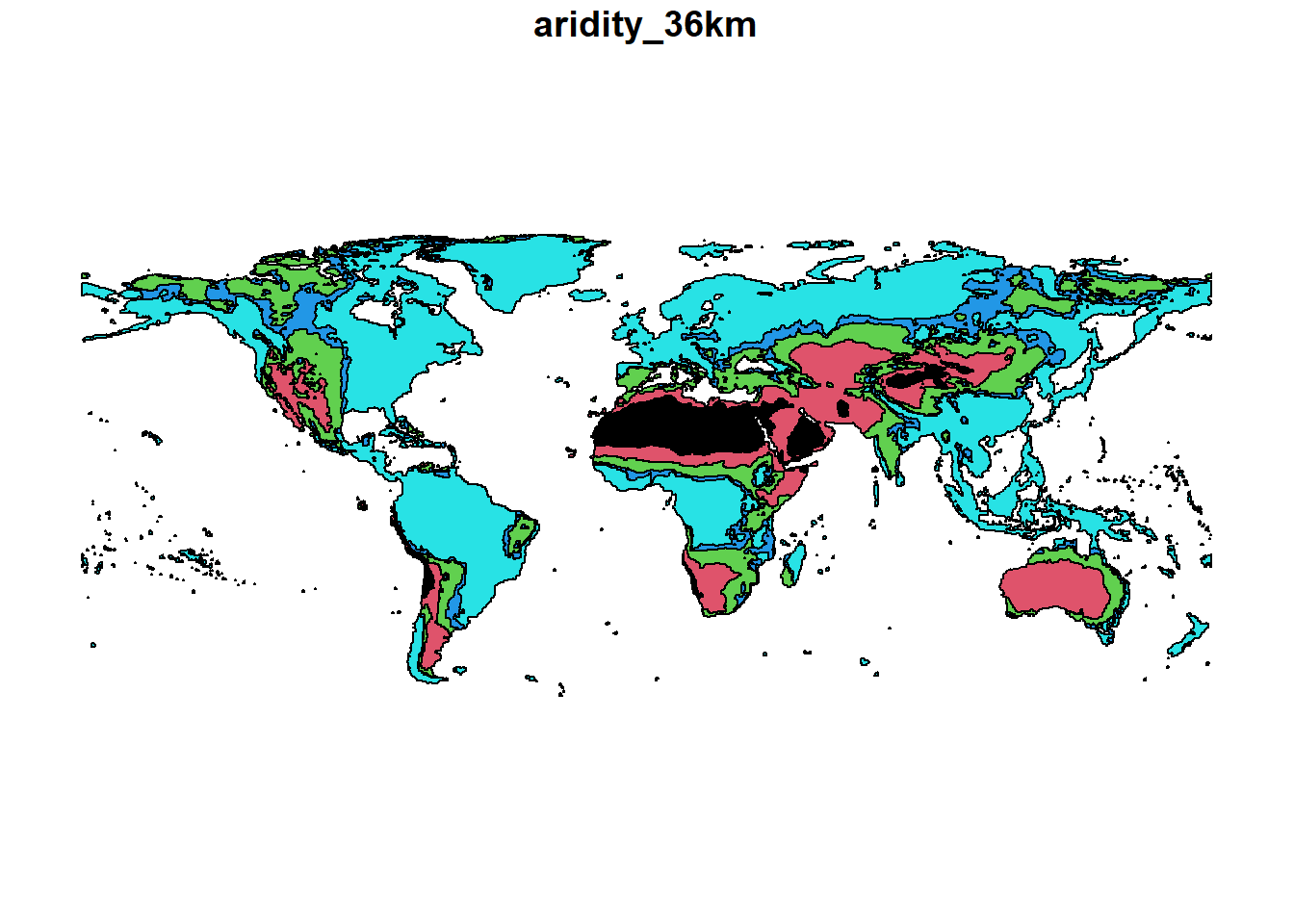
Summarize values of SMAP soil moisture raster for aridity classes:
sm_arid_df=terra::extract(sm,        # Raster to be summarized
                          vect(arid_poly), # Shapefile/ polygon to summarize the raster
                          fun=mean,  # Desired statistic: mean, sum, min and max
                          na.rm=TRUE)# Ignore NA values? yes!

# Lets plot the climate-wise mean of surface soil moisture
{plot(sm_arid_df,
     xaxt = "n",              # Disable x-tick labels
     xlab="Aridity",          # X axis label
     ylab="Soil moisture",    # Y axis label
     type="b",                # line type
     col="blue",              # Line color
     main="Climate-wise mean of surface soil moisture")
axis(1, at=1:5, labels=c("Hyper-arid", "Arid", "Semi-Arid","Sub-humid","Humid"))}