Chapter 3 Raster and shapefile visualization
A geographic information system, or GIS refers to a platform which can map, analyzes and manipulate geographically referenced dataset.
A geographically referenced data (or geo-referenced data) is a spatial dataset which can be related to a point on Earth with the help of geographic coordinates. Types of geo-referenced spatial data include: rasters (grids of regularly sized pixels) and vectors (polygons, lines, points).
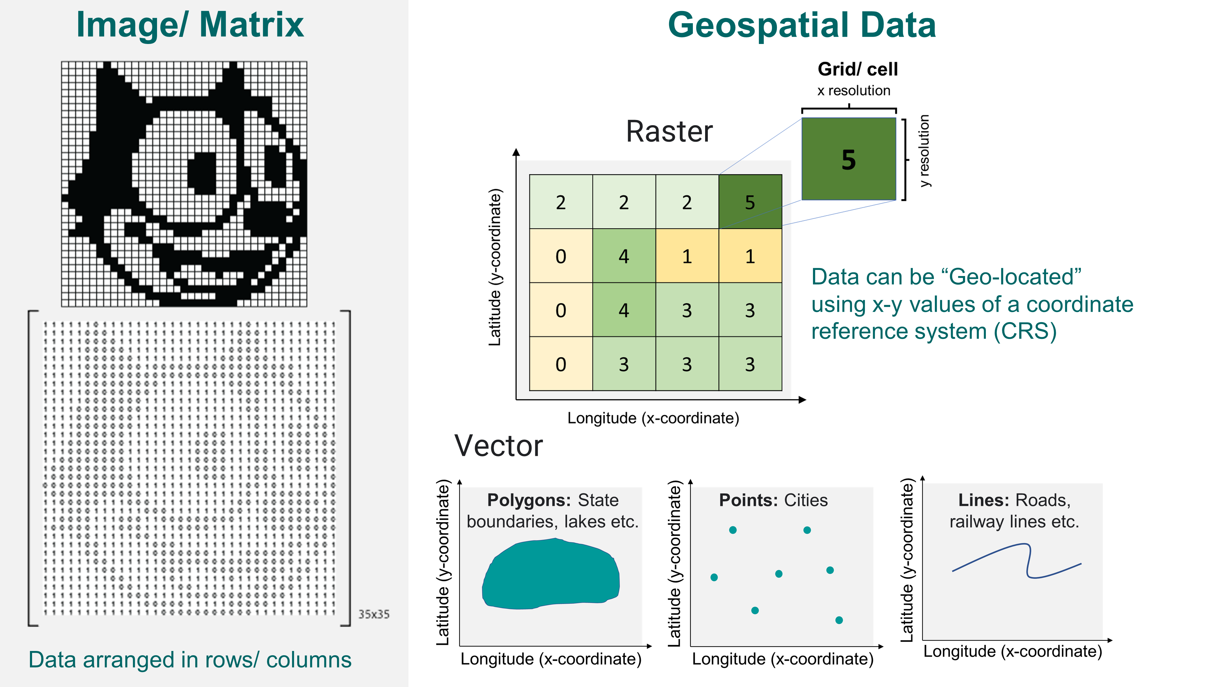
A quick and helpful review of spatial data can be found here: https://spatialvision.com.au/blog-raster-and-vector-data-in-gis/
3.1 Plotting raster data
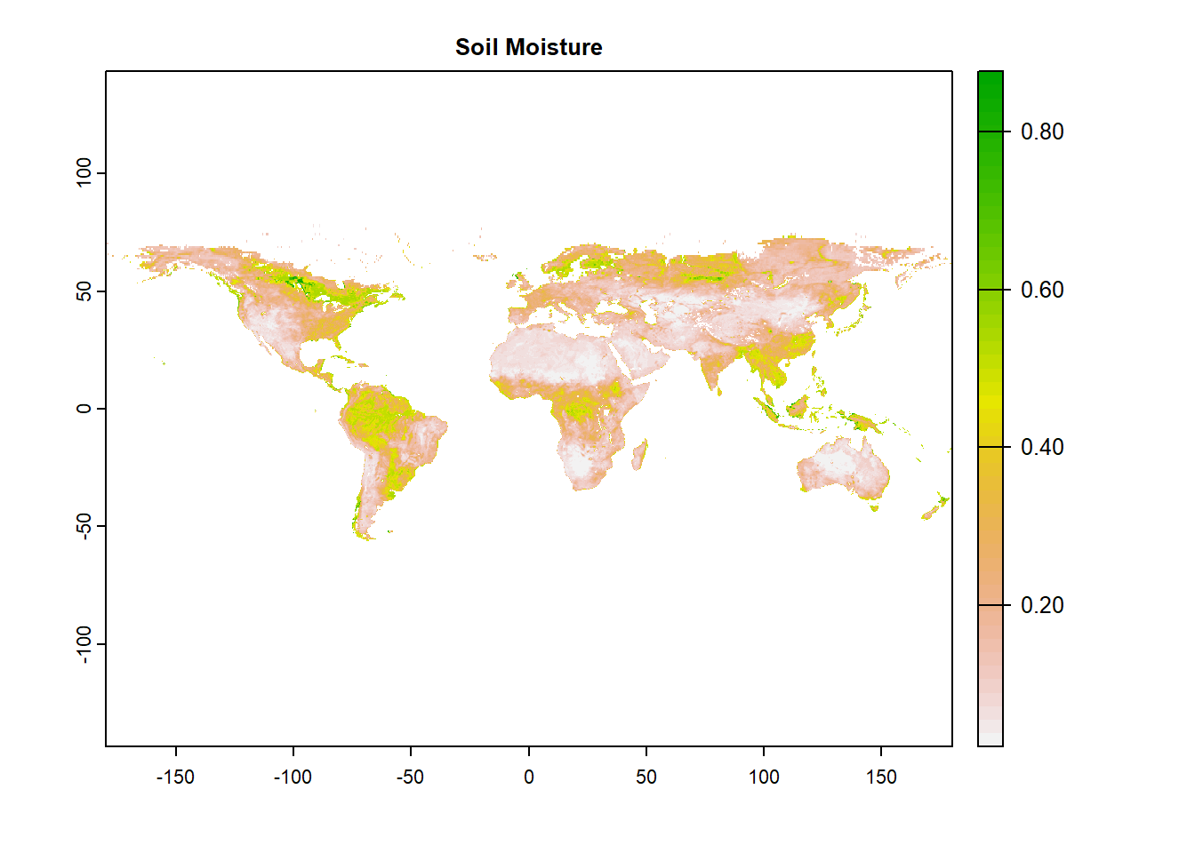
In this section, we will plot global raster data of surface (~5 cm) soil moisture from SMAP. In this process we will explore functions from terra, and tidyterra packages.
Let’s start by importing the necessary packages.
# For raster operations
library(terra)

# For plotting operations
library(tidyterra)
library(tmap)
library(ggplot2)
library(mapview)

# For Perceptually Uniform Colour palettes
library(cetcolor)
library(scico)

# Import SMAP soil moisture raster from the downloaded folder
sm=terra::rast("./SampleData-master/raster_files/SMAP_SM.tif")
Once we have imported the Spatraster using rast() function from terra package, let’s now check its attributes.
Notice the dimensions, resolution, extent, crs i.e. coordinate reference system and values. Note that the cell of one raster layer can only hold a single value. The value might be numeric or categorical!
## class       : SpatRaster
## dimensions  : 456, 964, 1  (nrow, ncol, nlyr)
## resolution  : 0.373444, 0.373444  (x, y)
## extent      : -180, 180, -85.24595, 85.0445  (xmin, xmax, ymin, ymax)
## coord. ref. : lon/lat WGS 84 (EPSG:4326)
## source      : SMAP_SM.tif
## name        :    SMAP_SM
## min value   : 0.01999998
## max value   : 0.87667608
# Try:
# dim(sm) # Dimension (nrow, ncol, nlyr) of the raster
# terra::res(sm) # X-Y resolution of the raster
# terra::ext(sm) # Spatial extent of the raster
# terra::crs(sm) # Coordinate reference systemNow let’s plot the raster using terra::plot. Interactive plots can be made by using mapview function.
 What are the different
 features of the above plot?
Expert Note: terra’s functionality is largely the same as the more mature raster package (created by the same developer, Robert Hijmans), but are usually more computationally efficient than raster equivalents. However, one can seamlessly translate between the two types of object to ensure backwards compatibility with older scripts and packages, for example, with the functions raster(), stack(), and brick() in the raster package.
3.2 Customizing terra plot options
3.2.1 Scientific Color palettes
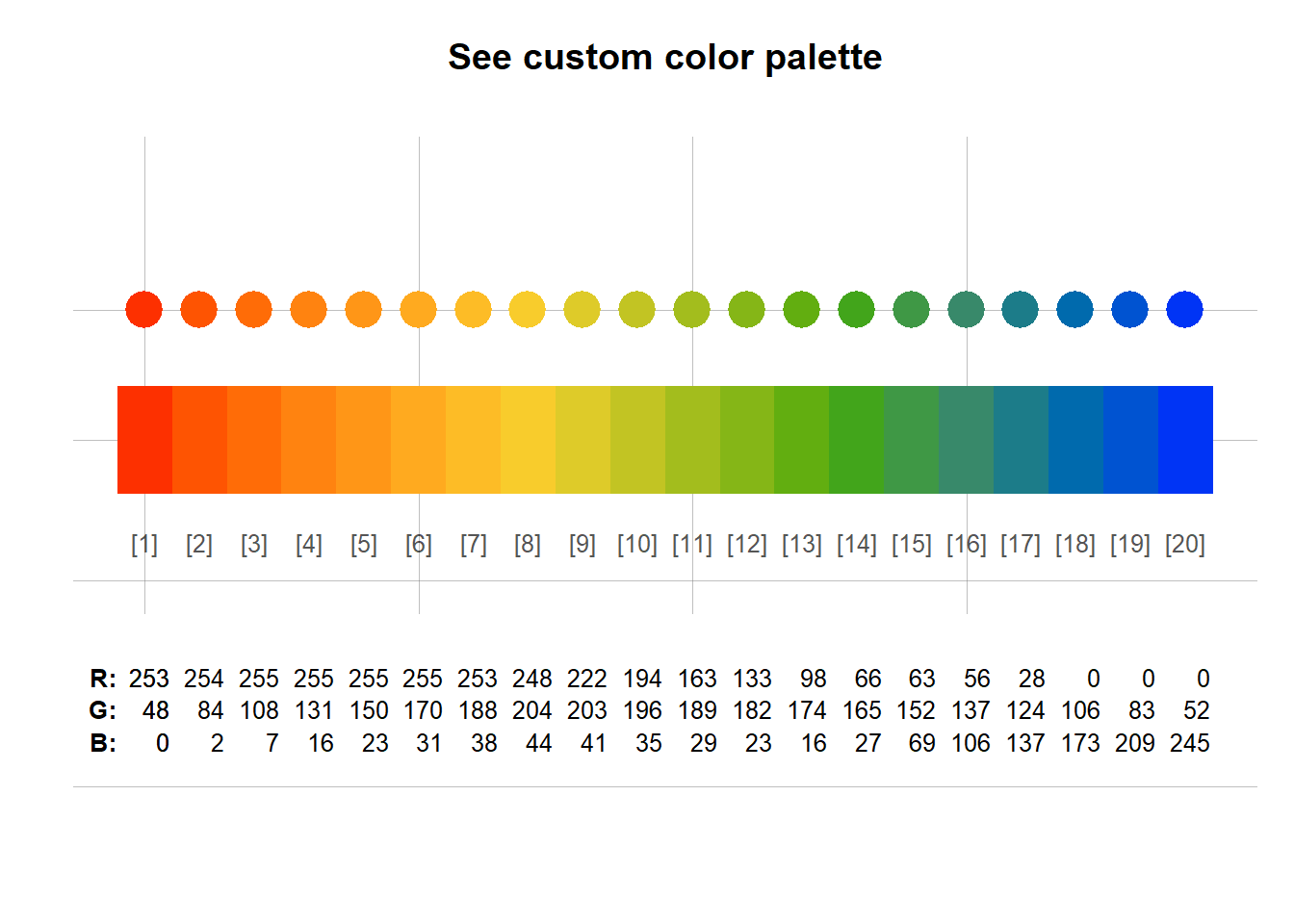
We will generate custom color palettes for better visualization. We will demonstrate the usage of cetcolor and scico package which provide access to the perceptually uniform and colour-blindness friendly palettes.
- You can select CET colormaps from: https://cran.r-project.org/web/packages/cetcolor/vignettes/cet_color_schemes.html
- You can select scico colormaps from: https://github.com/thomasp85/scico
- R Color Brewer is also a great resource for popular colormaps: https://colorbrewer2.org/#type=sequential&scheme=BuGn&n=3
# Make custom color palette
library(unikn)

#~~ A) User defined color palette using scico library
mypal1 = scico(20, alpha = 1.0, direction =  -1, palette = "vik")
unikn::seecol(mypal1)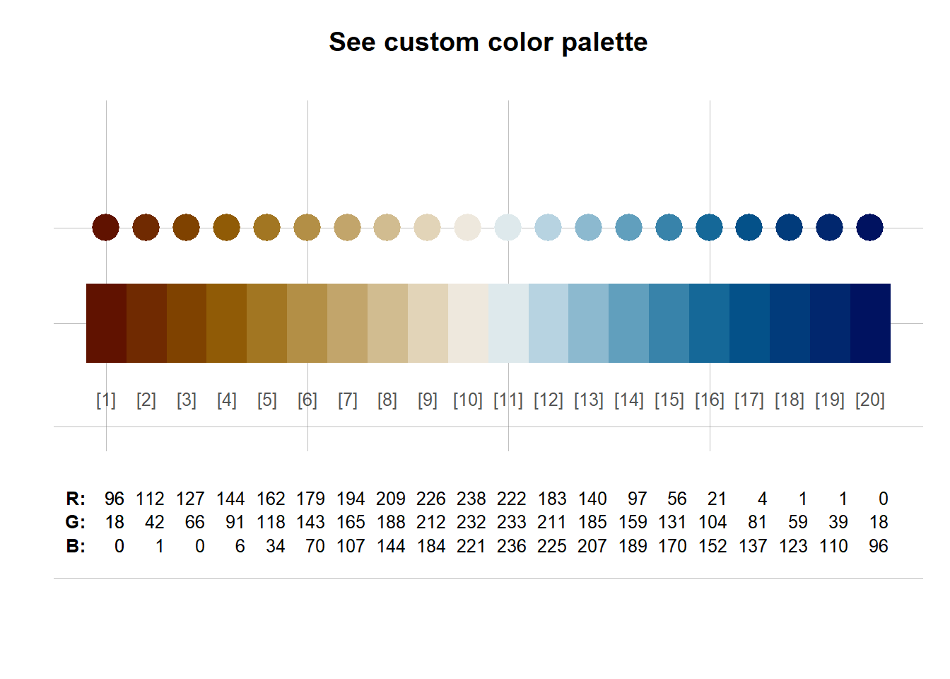
#Check: scico_palette_names() for available palettes!
# Try combinations of alpha=0.5, direction =1, and various different color palette

#~~ B) User defined color palette using cetcolor library
mypal2 = cetcolor::cet_pal(20, name = "r2")
unikn::seecol(mypal2)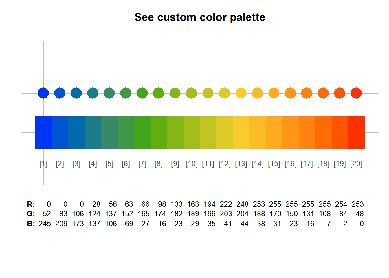
3.2.2 Customize terra plots
There is a long list of customizable operations available while plotting rasters in R. Let’s play with some of these options. We will start with basic plot from terra, and then venture into more powerful tmap and tidyterra packages.
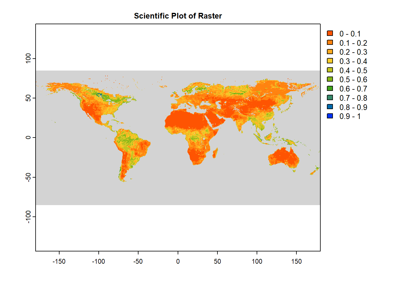
Try horizontal=TRUE, interpolate=FALSE, change xlim=c(-180, 180) with asp=1, or try legend.shrink=0.4.
sm=rast("./SampleData-master/raster_files/SMAP_SM.tif") # SMAP soil moisture data

terra::plot(sm,
            main = "Scientific Plot of Raster",

            #Color options
            col = mypal2,                    # User Defined Color Palette
            breaks = seq(0, 1, by=0.1),      # Sequence from 0-1 with 0.1 increment
            colNA = "lightgray",             # Color of cells with NA values

            # Axis options
            axes=TRUE,                       # Plot axes: TRUE/ FALSE
            xlim=c(-180, 180),               # X-axis limit
            ylim=c(-90, 90),                 # Y-axis limit
            xlab="Longitude",                # X-axis label
            ylab="Latitue",                  # Y-axis label

            # Legend options
            legend=TRUE,                     # Plot legend: TRUE/ FALSE

            # Miscellaneous
            mar = c(3.1, 3.1, 2.1, 7.1),     #Margins
            grid = FALSE                     #Add grid lines
        )
#Plotting through tmap:
tmap_mode("plot")  #Setting tmap mode: Static plots by "plot", Interactive plots by"view"

tmap_SM = tm_shape(sm)+
  tm_grid(alpha = 0.2)+
  tm_raster(alpha = 0.7, palette = mypal2,
            style = "pretty", title = "Volumetric Soil Moisture")+
  tm_layout(legend.position = c("left", "bottom"))+
  tm_xlab("Longitude")+ tm_ylab("Latitude")

tmap_SM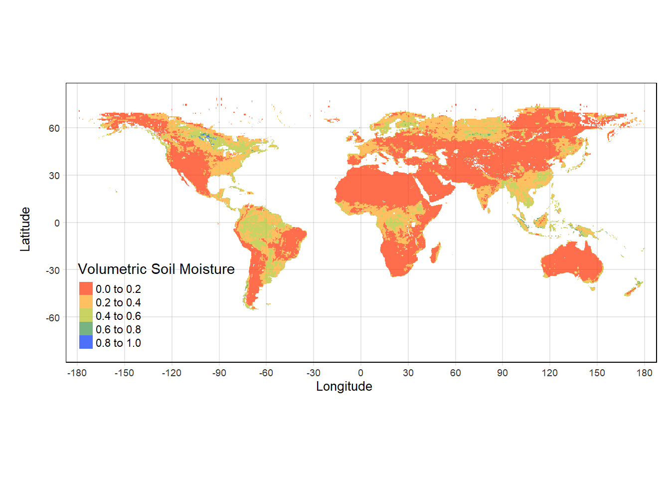
To convert the static plot into an interactive map we will use mapview package which which is compatible with rasterbrick.
# Interactive plot
library(mapview)
library(raster)

mapview(brick(sm),            # Convert SpatRaster to RasterBrick
        col.regions = mypal2, # Color palette
        at=seq(0, 0.8, 0.1)   # Breaks
        )
Other examples for using interactive plots with mapview can be found at: https://vinit-sehgal.github.io/AGRO4092/ch10.html#exercise-4
3.3 Plotting raster data using tidyterra
tidyterra is a package that add common methods from the tidyverse for SpatRaster and SpatVectors objects created with the {terra} package. It also adds specific geom_spat*() functions for plotting these kind of objects with {ggplot2}.
Note on Performance: tidyterra is conceived as a user-friendly wrapper of {terra} using the {tidyverse} methods and verbs. This approach therefore has a cost in terms of performance.
library(tidyterra)
library(ggplot2)

ggplot() +
  geom_spatraster(data = sm) +
  scale_fill_gradientn(colors=mypal2,                               # Use user-defined colormap
                       name = "SM",                                 # Name of the colorbar
                       na.value = "transparent",                    # transparent NA cells
                       labels=(c("0", "0.2", "0.4", "0.6", "0.8")), # Labels of colorbar
                       breaks=seq(0,0.8,by=0.2),                    # Set breaks of colorbar
                       limits=c(0,0.8))+
  theme_void()  # Try different themes: theme_bw(), theme_gray(), theme_minimal()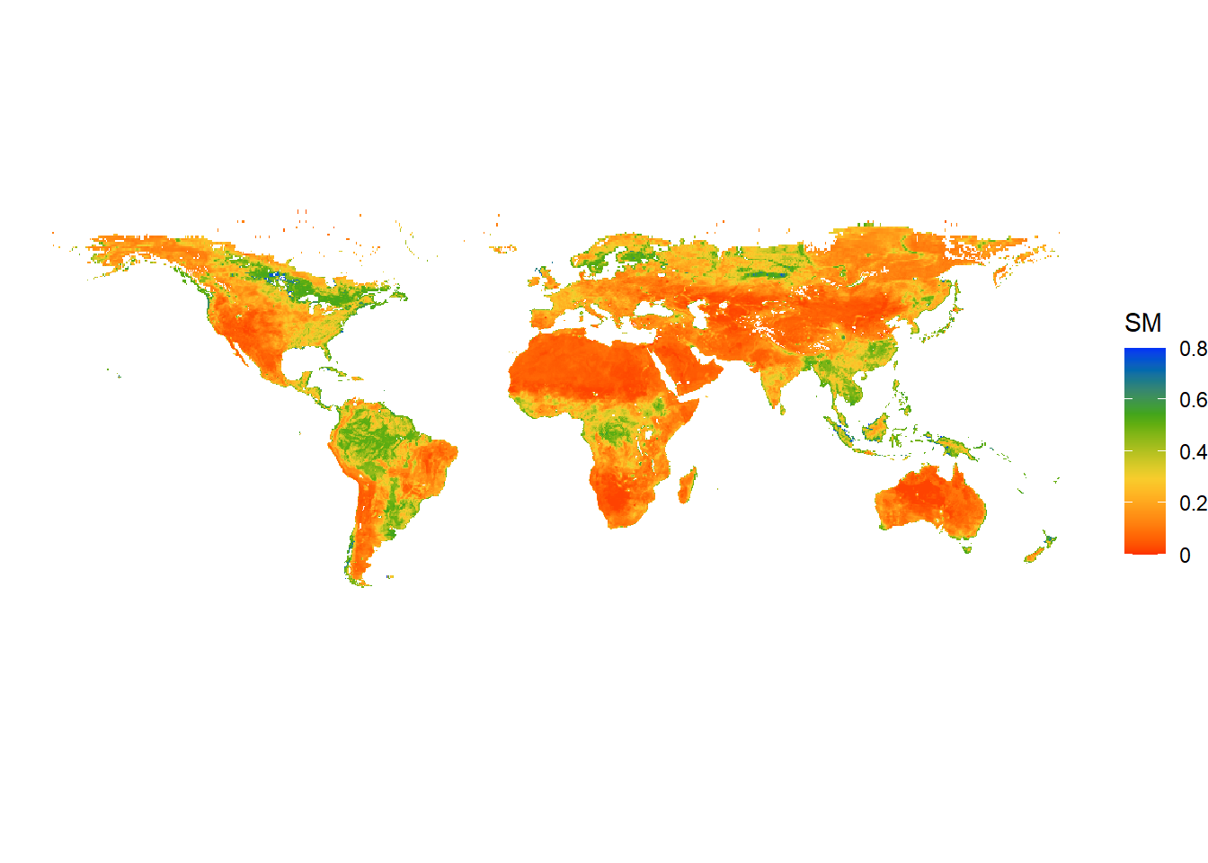
What if we are interested in a particular region and not the entire globe? We can plot the map for a specific extent (CONUS, in this case) by changing the range of coord_sfoption. We will also use a different theme: theme_bw. Try xlim = c(114,153) and ylim = c(-43,-11)!
sm_conus= ggplot() +
  geom_spatraster(data = sm) +
  scale_fill_gradientn(colors=mypal2,                               # Use user-defined colormap
                       name = "SM",                                 # Name of the colorbar
                       na.value = "transparent",                    # transparent NA cells
                       labels=(c("0", "0.2", "0.4", "0.6", "0.8")), # Labels of colorbar
                       breaks=seq(0,0.8,by=0.2),                    # Set breaks of colorbar
                       limits=c(0,0.8)) +
  coord_sf(xlim = c(-125,-67),                                      # Add extent for CONUS
              ylim = c(24,50))+
  theme_bw()                                                        # Try black-and-white theme.

print(sm_conus)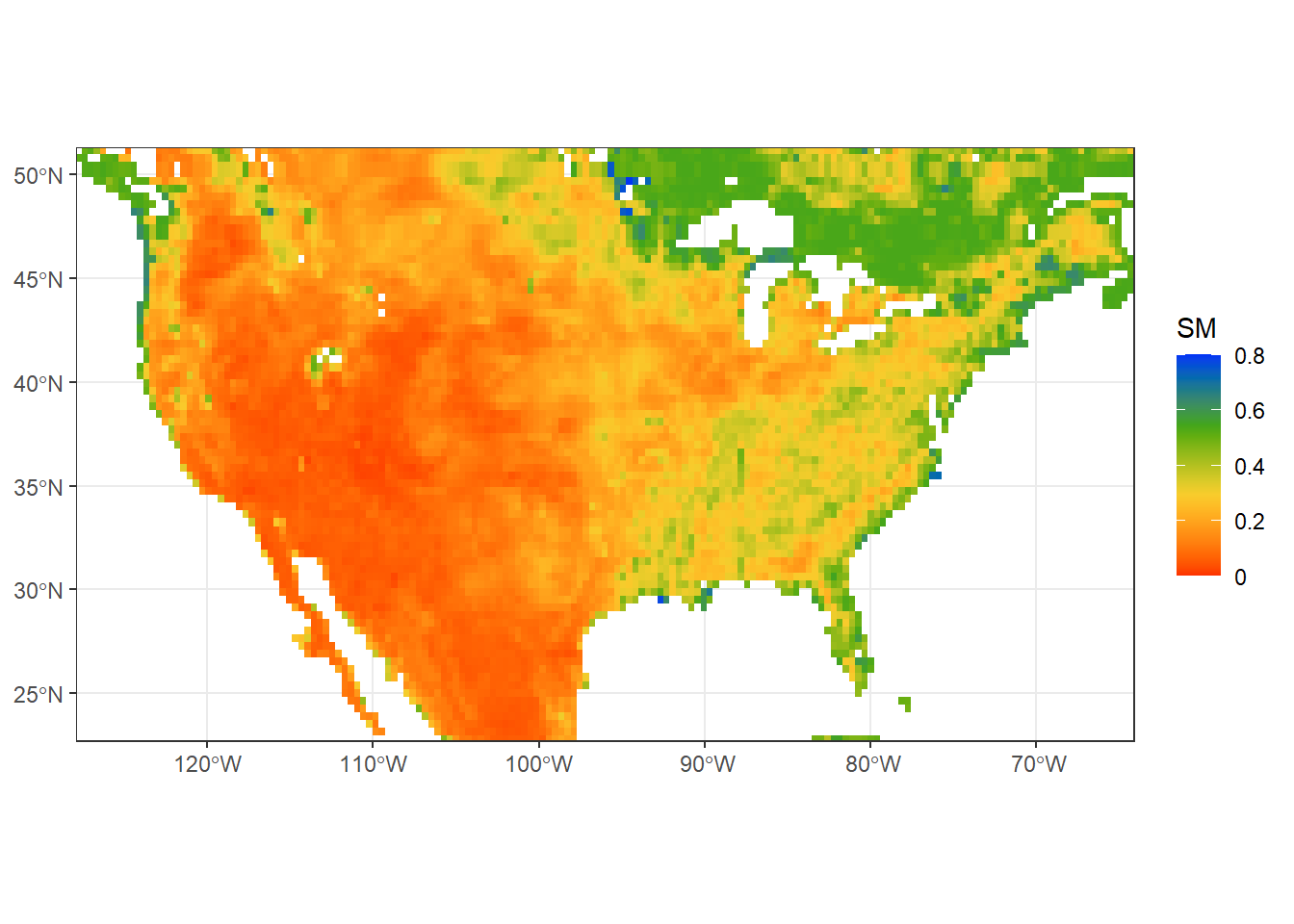
tmap provides the easiest way of manipulating the legends from continuous to discrete by just adding the style of color scale desired by the user.
#We will manipulate the existing tmap_SM plot by adding style parameter:
tmap_SM = tm_shape(sm)+
  tm_grid(alpha = 0.2)+
  tm_raster(alpha = 0.7, style = "pretty",
            palette = mypal2,  title = "Volumetric Soil Moisture") +
  tm_layout(legend.position = c("left","bottom"), inner.margins = 0)+           #Adjust the legend position
   tm_xlab("Longitude")+ tm_ylab("Latitude")

tmap_SM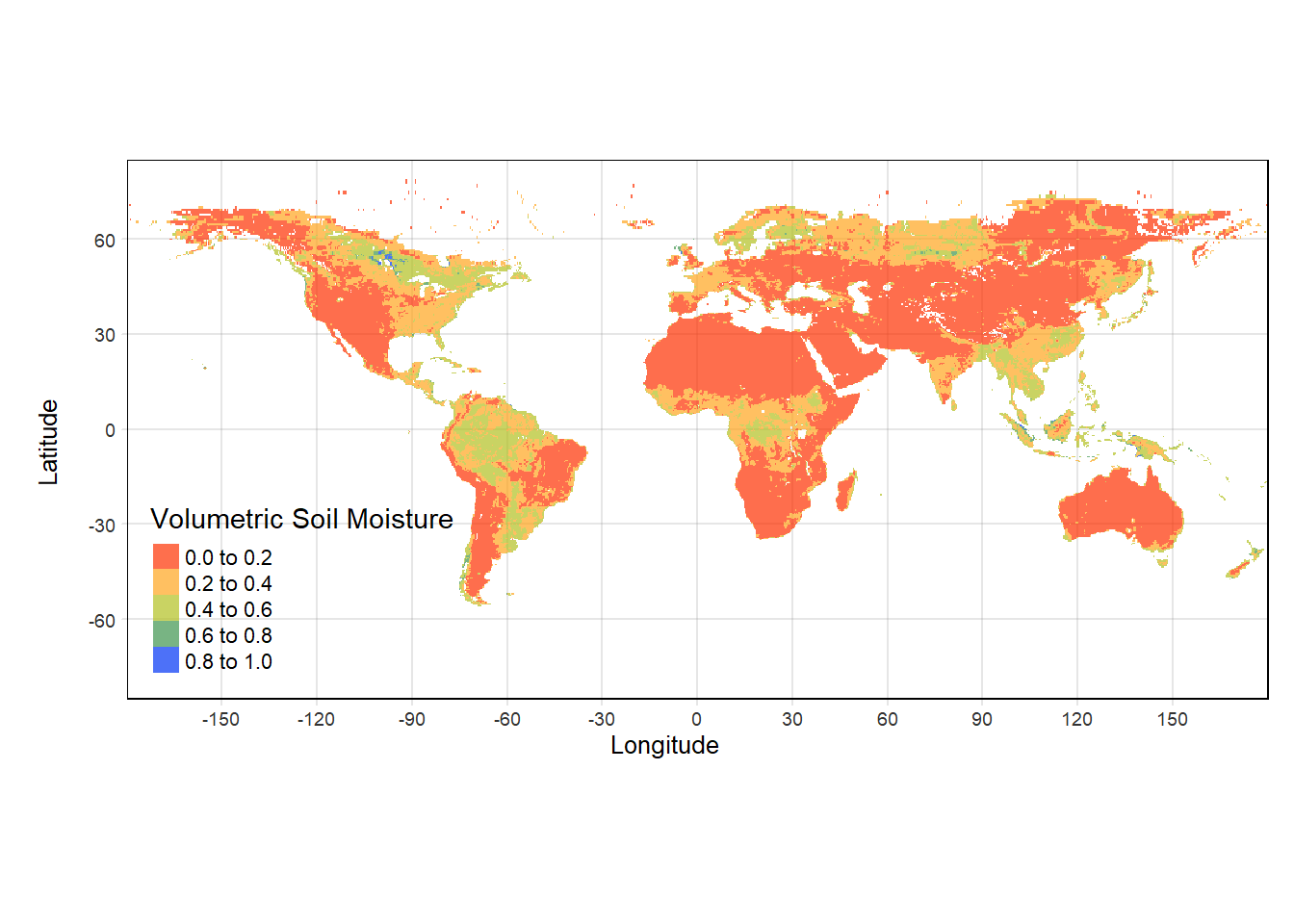
#Using breaks would give more control on scale discretization
tm_shape(sm)+
  tm_grid(alpha = 0.2)+
  tm_raster(alpha = 0.7, breaks = c(0.00, 0.25, 0.50, 0.75, 1.00),
            palette = mypal2,  title = "Volumetric Soil Moisture") +
  tm_layout(legend.outside = TRUE,
            legend.outside.position = c("right","top"),
            inner.margins = 0)+
  tm_xlab("Longitude")+ tm_ylab("Latitude")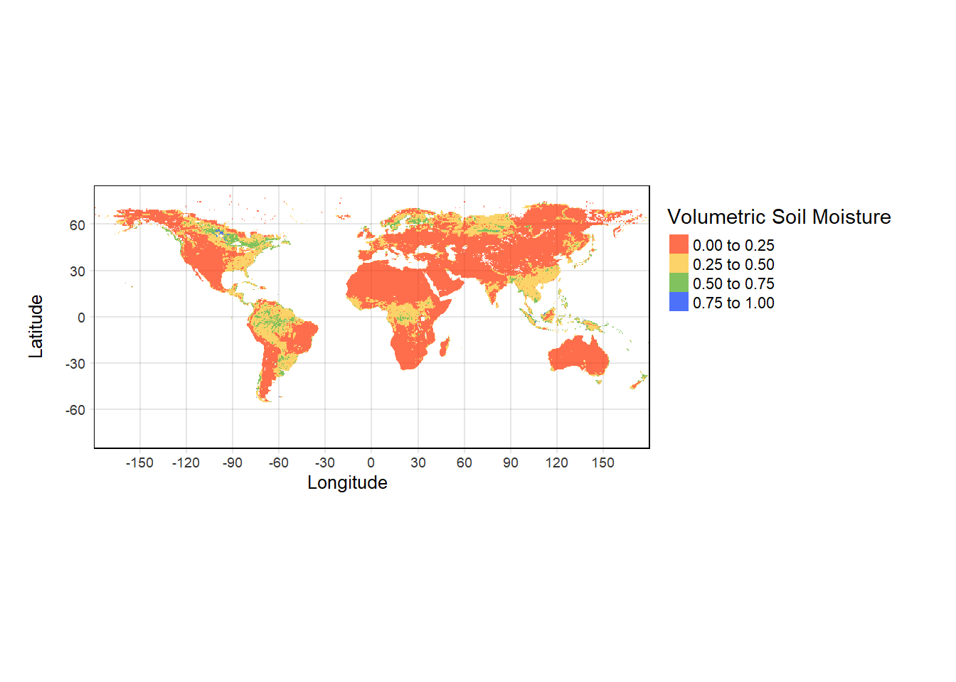
3.4 Plotting vector data
Importing and plotting shapefiles is equally easy in R. We will import the shapefile of the updated global IPCC climate reference regions (https://doi.org/10.5194/essd-12-2959-2020) as Simple Feature (sf) Object. We will also use global coastline shapefile from the web for plotting.
Note: Even though terra provides vect() function to handle vector data, sf package is most suitable and powerful for manipulating and plotting purposes.
###############################################################
#~~~  Importing and visualizing shapefiles
library(sf)

# Import the shapefile of global IPCC climate reference regions (only for land)
IPCC_shp = read_sf("./SampleData-master/CMIP_land/CMIP_land.shp")

# View attribute table of the shapefile
IPCC_shp # Notice the attributes look like a data frame
## Simple feature collection with 41 features and 4 fields
## Geometry type: POLYGON
## Dimension: XY
## Bounding box: xmin: -168 ymin: -56 xmax: 180 ymax: 85
## Geodetic CRS: WGS 84
## # A tibble: 41 × 5
## V1 V2 V3 V4 geometry
## <chr> <chr> <chr> <dbl> <POLYGON [°]>
## 1 ARCTIC Greenland/Iceland GIC 1 ((-10 58, -10.43956 58, -10.87…
## 2 NORTH-AMERICA N.E.Canada NEC 2 ((-55 50, -55.4386 50, -55.877…
## 3 NORTH-AMERICA C.North-America CNA 3 ((-90 50, -90 49.5614, -90 49.…
## 4 NORTH-AMERICA E.North-America ENA 4 ((-70 25, -70.43478 25, -70.86…
## 5 NORTH-AMERICA N.W.North-America NWN 5 ((-105 50, -105.4386 50, -105.…
## 6 NORTH-AMERICA W.North-America WNA 6 ((-130 50, -129.5614 50, -129.…
## 7 CENTRAL-AMERICA N.Central-America NCA 7 ((-90 25, -90.37179 24.76923, …
## 8 CENTRAL-AMERICA S.Central-America SCA 8 ((-75 12, -75.28 11.67333, -75…
## 9 CENTRAL-AMERICA Caribbean CAR 9 ((-75 12, -75.32609 12.28261, …
## 10 SOUTH-AMERICA N.W.South-America NWS 10 ((-75 12, -74.57143 12, -74.14…
## # ℹ 31 more rows# Load global coastline shapefile
coastlines = read_sf("./SampleData-master/ne_10m_coastline/ne_10m_coastline.shp")
# Alternatively, download global coastlines from the web
# NOTE: May not work if the online server is down
# download.file("https://www.naturalearthdata.com/http//www.naturalearthdata.com/download/110m/physical/ne_110m_coastline.zip?version=4.0.1",destfile = 'ne_110m_coastline.zip')
# # Unzip the downloaded file
# unzip(zipfile = "ne_110m_coastline.zip",exdir = 'ne-coastlines-110m')
# Plot both sf objects using tmap:
tm_shape(IPCC_shp)+
tm_borders()+ # Add IPCC land regions in blue color
tm_shape(coastlines)+
tm_sf() # Add global coastline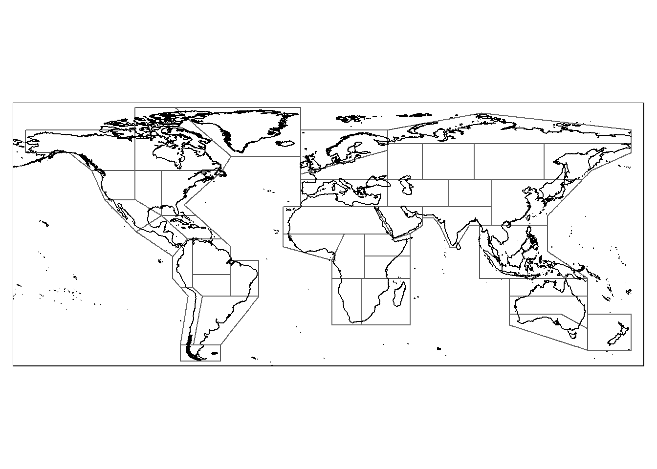
#Subset shapefile for Eastern North-America
terra::plot(IPCC_shp[4,][1], main="Polygon for Eastern North-America")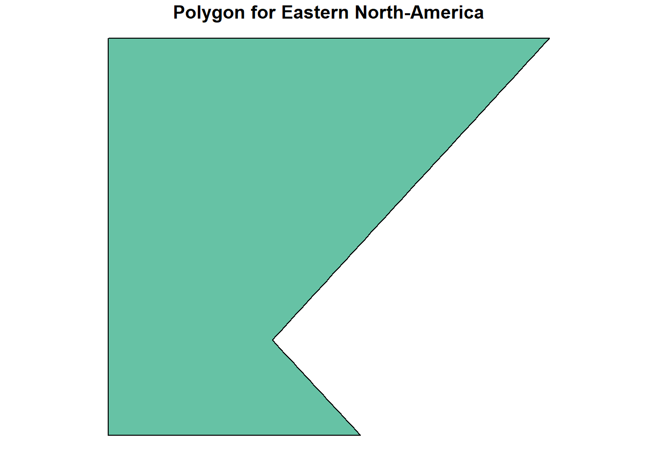
# Combine terra plots with overlaying shapefiles
tmap_SM +
  tm_shape(IPCC_shp)+
  tm_borders()+
  tm_shape(coastlines)+
  tm_sf()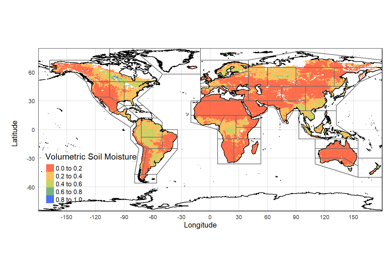
###############################################################
#~~~ Add spatial point to shapefile/ raster
#~~ Create a spatial point for College Station, Texas
college_station = st_sfc(
st_point(x = c(-96.33, 30.62), dim = "XY"), # Lat-long as spatial points
crs = "EPSG:4326") # Coordinate system: More details in the next part
#~~ Create map by adding all the layers
tm_shape(IPCC_shp[c(3,4,6,7),])+ # Selected regions from 'IPCC_shp'
tm_borders(col = "black",lwd = 1, lty = "solid")+ # Border color
tm_fill(col = "lightgrey")+ # Fill color
tm_shape(coastlines)+ # Add coastline
tm_sf(col = "maroon")+ # Change color of coastline
tm_shape(college_station)+ # Add spatial point to the map
tm_dots(size = 2, col = "blue") # Customize point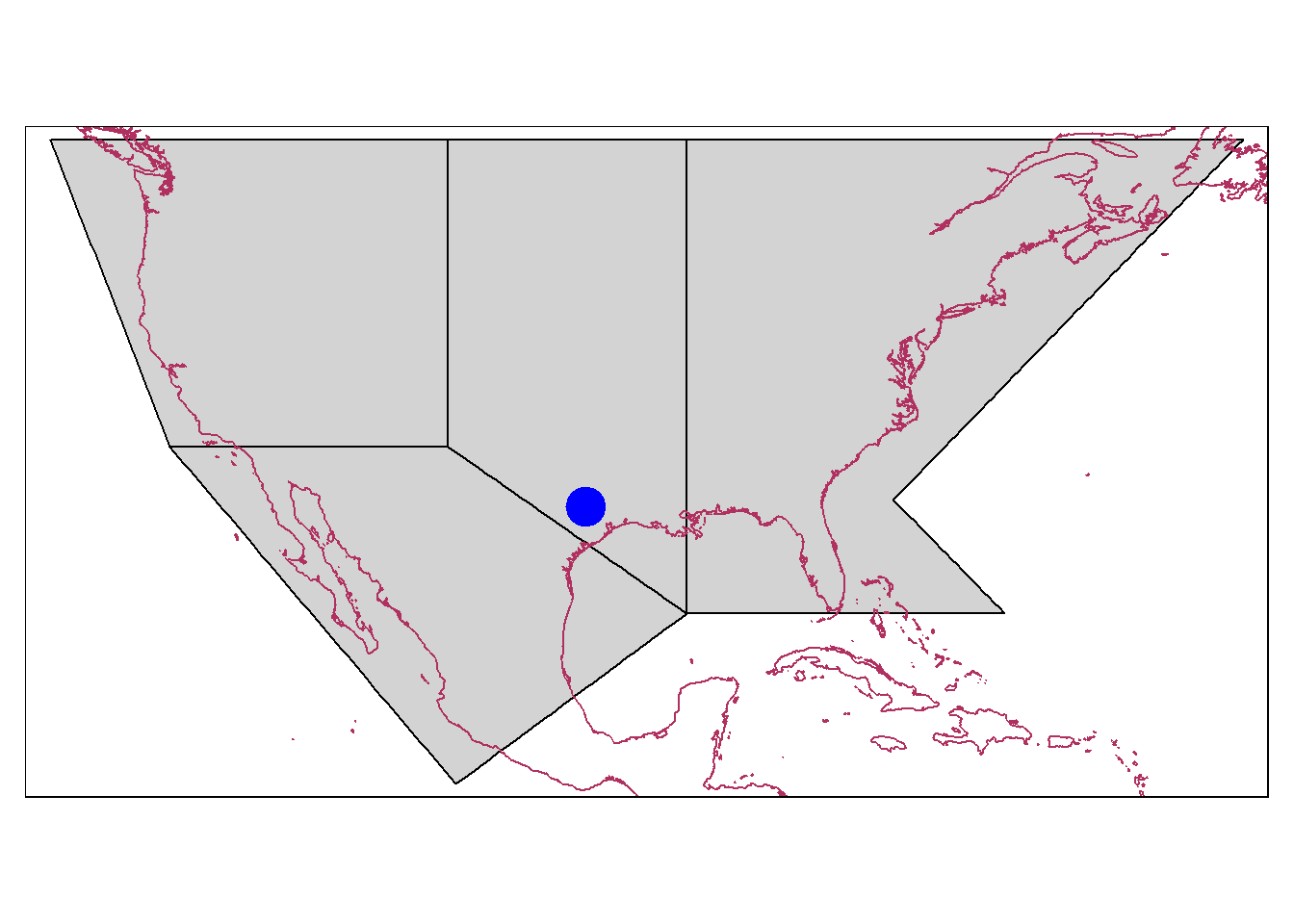 Note: Each layer (here 3) needs to be added as with tm_shape()!
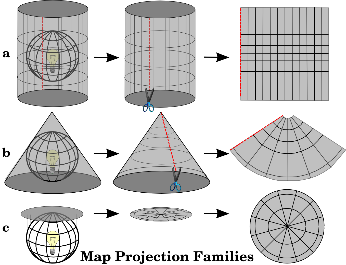
3.5 Reprojection of rasters using terra::project
A coordinate reference system (CRS) is used to relate locations on Earth (which is a 3-D spheroid) to a 2-D projected map using coordinates (for example latitude and longitude). Projected CRSs are usually expressed in Easting and Northing (x and y) values corresponding to long-lat values in Geographic CRS. A good description of coordinate reference systems and their importance can be found here: https://docs.qgis.org/3.4/en/docs/gentle_gis_introduction/coordinate_reference_systems.html https://datacarpentry.org/organization-geospatial/03-crs/
In R, the coordinate reference systems or CRS are commonly specified in EPSG (European Petroleum Survey Group) or PROJ4 format (See: https://epsg.io/).
The Spatraster reprojection process is done with project() from the terra package.
# Importing SMAP soil moisture data
sm=rast("./SampleData-master/raster_files/SMAP_SM.tif")

#~~ Projection 1: NAD83 (EPSG: 4269)

sm_proj1 = terra::project(sm, "epsg:4269")

terra::plot(sm_proj1,
             main = "NAD83",    # Title of the plot
             col = mypal2,      # Colormap for the plot
             axes = FALSE,      # Disable axes
             box = FALSE,       # Disable box around the plots
             asp = NA,          # No fixed aspect ratio; asp=NA fills plot to window
             legend=FALSE)      # Disable legend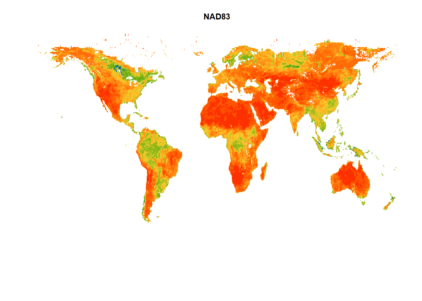
#~~ Projection 2: World Robinson projection (ESRI:54030)

sm_proj2 = terra::project(sm, "ESRI:54030")

terra::plot(sm_proj2,
             main = "Robinson", # Title of the plot
             col = mypal2,      # Colormap for the plot
             axes = FALSE,      # Disable axes
             box = FALSE,       # Disable box around the plots
             asp = NA,          # No fixed aspect ratio; asp=NA fills plot to window
             legend=FALSE)      # Disable legend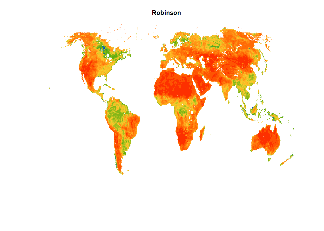
Other than the projections demonstrated, try the following:
"+init=epsg:3857" For Mercator (EPSG: 3857): Used in Google Maps, Open Street Maps, etc.
"+proj=robin +lon_0=0 +x_0=0 +y_0=0 +ellps=WGS84 +datum=WGS84 +units=m +no_defs" for World Robinson Projection
"+proj=merc +lon_0=0 +k=1 +x_0=0 +y_0=0 +ellps=WGS84 +datum=WGS84 +units=m +no_defs" for World Mercator projection
We will use a custom function provided with the material to plot the global raster in Robinson projection.
#~~~Projection 2: Robinson projection
WorldSHP=terra::vect(spData::world)
RobinsonPlot <- ggplot() +
geom_spatraster(data = sm)+ # Plot SpatRaster layer
geom_spatvector(data = WorldSHP,
fill = "transparent") + # Add world political map
ggtitle("Robinson Projection") + # Add title
scale_fill_gradientn(colors=mypal2, # Use user-defined colormap
name = "Soil Moisture", # Name of the colorbar
na.value = "transparent",# Set color for NA values
lim=c(0,0.8))+ # Z axis limit
theme_minimal()+ # Select theme. Try 'theme_void'
theme(plot.title = element_text(hjust =0.5), # Place title in the middle of the plot
text = element_text(size = 12))+ # Adjust plot text size for visibility
coord_sf(crs = "ESRI:54030", # Reproject to World Robinson
xlim = c(-152,152)*100000,
ylim = c(-55,90)*100000)
print(RobinsonPlot)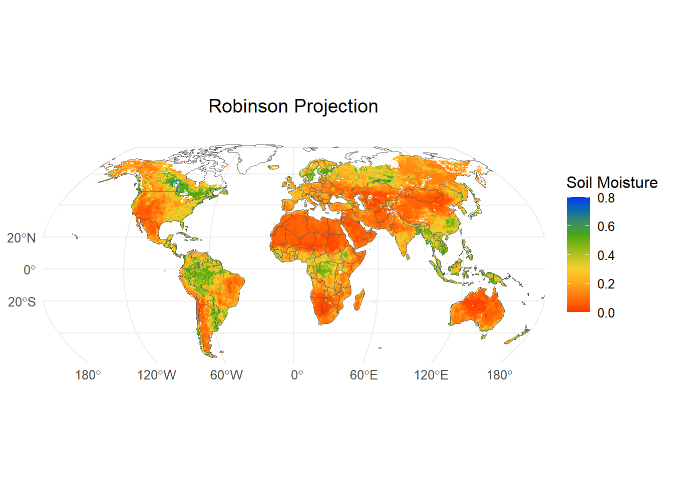 Now let’s plot the
 robison plot using tmap:
WorldSHP = st_as_sf(WorldSHP)           # Convert 'WorldSHP' to simple feature

tm_shape(WorldSHP,                      # Initiate shapefile
         projection = 'ESRI:54030',     # Set projection: World Robinson
         ylim = c(-65, 90)*100000,      # Set y-limit
         xlim = c(-152,152)*100000,     # Set x-limit
         raster.warp = TRUE)+
  tm_sf()+                              # Plot shapefile
  tm_shape(sm,                          # Add raster file
           projection = 'ESRI:54030',   # Set projection
           raster.warp = FALSE) +
  tm_raster( palette = mypal2,          # Set color map for raster
             title = "Soil Moisture")+  # Add plot title
  tm_layout(main.title = "Surface Soil Moisture",
            main.title.fontfamily = "Times",               # Set text font
            legend.show = T,                               # Show legend= T/F
            legend.outside = T,
            legend.outside.position = c("right", "top"),   # Legend position
            frame = FALSE,                                 # Add plot frame
            earth.boundary.color = "grey",                 # Boundary color
            earth.boundary.lwd = 2,                        # Boundary linewidth
            fontfamily = "Times")+                         # Text font
  tm_graticules(alpha = 0.2,                               # Add lat-long graticules
                labels.inside.frame = FALSE,
                col = "lightgrey", n.x = 4, n.y = 3)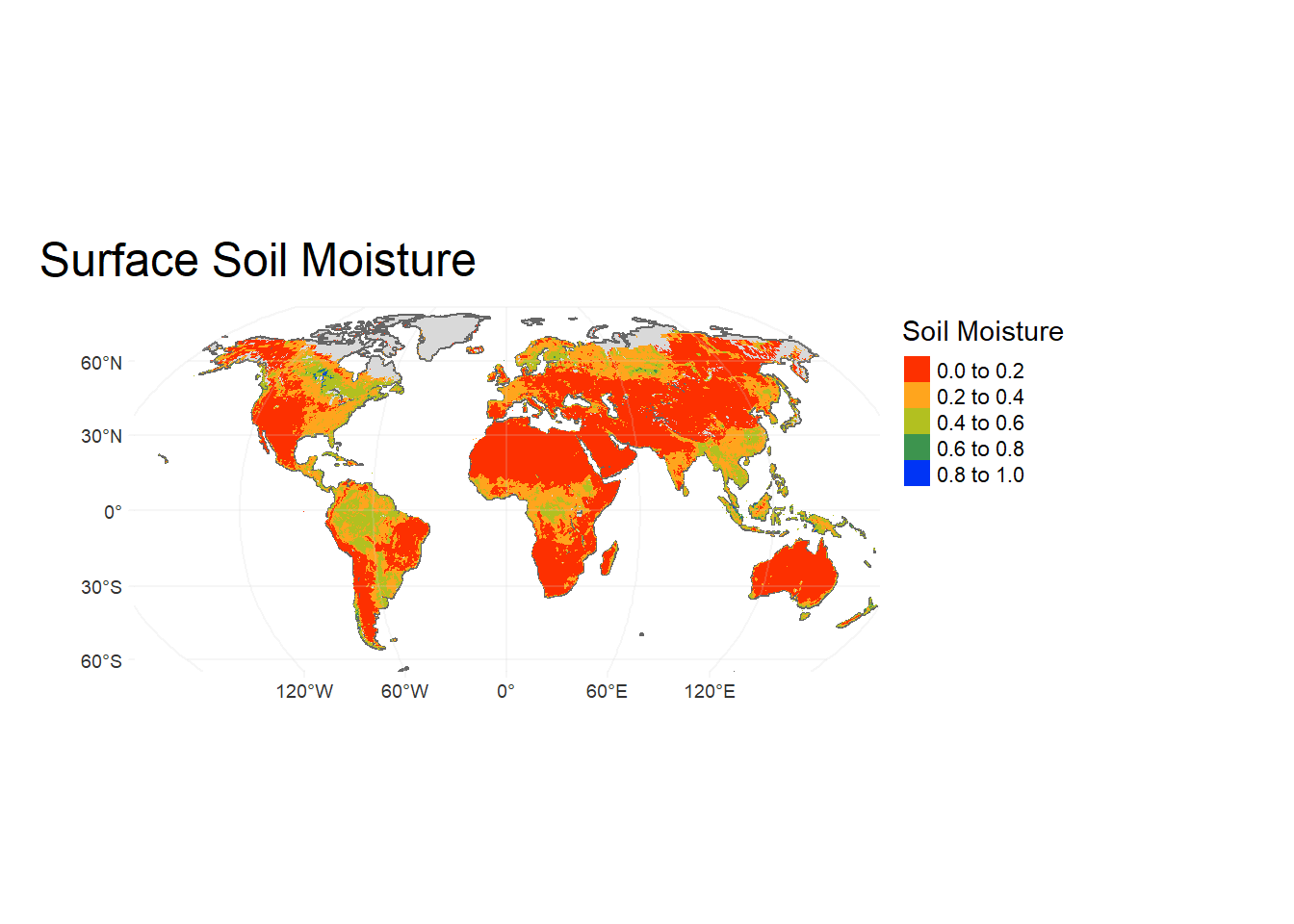
Useful references: More excellent examples on making maps in R can be found here: https://bookdown.org/nicohahn/making_maps_with_r5/docs/introduction.html. Quintessential resource for reference on charts and plots in R: https://www.r-graph-gallery.com/index.html.