The U.S. Climate Reference Network (USCRN) is a systematic and sustained network of climate monitoring stations. USCRN has sites across Contiguous U.S. along with some in Alaska, and Hawaii. These stations are instrumented to measure meteorological information such as temperature, precipitation, wind speed, along with other relevant hydrologic variables such as soil moisture at uniform depths (5, 10, 20, 50, 100 cm) at sub-hourly, daily and monthly time scales. Users can access daily data set from all station suing the following link: Index of /pub/data/uscrn/products/daily01 (noaa.gov)
Let us extract sample data from a USCRN site in Lafayette, LA, USA for 2021.
# Yearly data from the sample stationutils::download.file("https://github.com/Vinit-Sehgal/AGRO4092/blob/main/SampleData-master/CRN_data/CRND0103-2021-OK_Stillwater_2_W.txt?raw=true",destfile ="CRND0103-2021-OK_Stillwater_2_W.txt", mode="wb", #wb is write binarymethod ='auto', quiet=FALSE)utils::download.file("https://github.com/Vinit-Sehgal/AGRO4092/blob/main/SampleData-master/CRN_data/HEADERS.txt?raw=true",destfile ="headers.txt", mode="wb", #wb is write binarymethod ='auto', quiet=FALSE)CRNdat =read.csv("CRND0103-2021-OK_Stillwater_2_W.txt", header=FALSE,sep="")headers =read.csv("headers.txt", header=FALSE,sep="")# OR Direct download from NCEI servers (might not work during server downtime)#CRNdat = read.csv(url("https://www.ncei.noaa.gov/pub/data/uscrn/products/daily01/2021/CRND0103-2021-OK_Stillwater_2_W.txt"), header=FALSE,sep="")# Data headers#headers=read.csv(url("https://www.ncei.noaa.gov/pub/data/uscrn/products/daily01/headers.txt"), header=FALSE,sep="")# Column names as headers from the text filecolnames(CRNdat)=headers[2,1:ncol(CRNdat)]# Replace fill values with NACRNdat[CRNdat ==-9999]=NACRNdat[CRNdat ==-99]=NACRNdat[CRNdat ==999]=NA# View data samplelibrary(kableExtra)dataTable =kbl(head(CRNdat,6),full_width = F)kable_styling(dataTable,bootstrap_options =c("striped", "hover", "condensed", "responsive"))
WBANNO
LST_DATE
CRX_VN
LONGITUDE
LATITUDE
T_DAILY_MAX
T_DAILY_MIN
T_DAILY_MEAN
T_DAILY_AVG
P_DAILY_CALC
SOLARAD_DAILY
SUR_TEMP_DAILY_TYPE
SUR_TEMP_DAILY_MAX
SUR_TEMP_DAILY_MIN
SUR_TEMP_DAILY_AVG
RH_DAILY_MAX
RH_DAILY_MIN
RH_DAILY_AVG
SOIL_MOISTURE_5_DAILY
SOIL_MOISTURE_10_DAILY
SOIL_MOISTURE_20_DAILY
SOIL_MOISTURE_50_DAILY
SOIL_MOISTURE_100_DAILY
SOIL_TEMP_5_DAILY
SOIL_TEMP_10_DAILY
SOIL_TEMP_20_DAILY
SOIL_TEMP_50_DAILY
SOIL_TEMP_100_DAILY
53926
20210101
2.622
-97.09
36.12
2.1
0.2
1.2
0.8
23.0
3.51
C
1.0
-0.3
0.3
93.1
70.1
86.2
0.474
0.440
0.458
0.450
0.429
3.9
4.2
5.4
8.3
9.9
53926
20210102
2.622
-97.09
36.12
6.9
-2.5
2.2
1.8
0.0
7.02
C
9.9
-4.7
1.1
94.2
57.3
78.7
0.466
0.443
0.459
0.448
0.432
4.6
4.7
5.5
8.0
9.6
53926
20210103
2.622
-97.09
36.12
9.1
-3.7
2.7
1.3
0.0
10.56
C
12.9
-6.2
-0.2
94.2
56.4
83.5
0.436
0.440
0.460
0.449
0.429
4.2
4.7
5.5
7.8
9.4
53926
20210104
2.622
-97.09
36.12
14.7
-3.2
5.7
4.3
0.0
11.13
C
16.8
-6.0
2.0
94.0
46.2
76.4
0.423
0.428
0.461
0.450
0.430
4.6
5.0
5.6
7.6
9.2
53926
20210105
2.622
-97.09
36.12
16.2
-3.6
6.3
6.2
0.0
9.99
C
17.9
-6.5
3.9
94.0
22.0
59.5
0.412
0.417
0.463
0.453
0.431
4.8
5.2
5.7
7.6
9.1
53926
20210106
2.622
-97.09
36.12
9.6
4.8
7.2
7.5
0.3
1.03
C
11.4
4.3
7.1
92.1
45.8
66.7
0.395
0.412
0.459
0.450
0.431
6.2
6.1
6.2
7.6
9.1
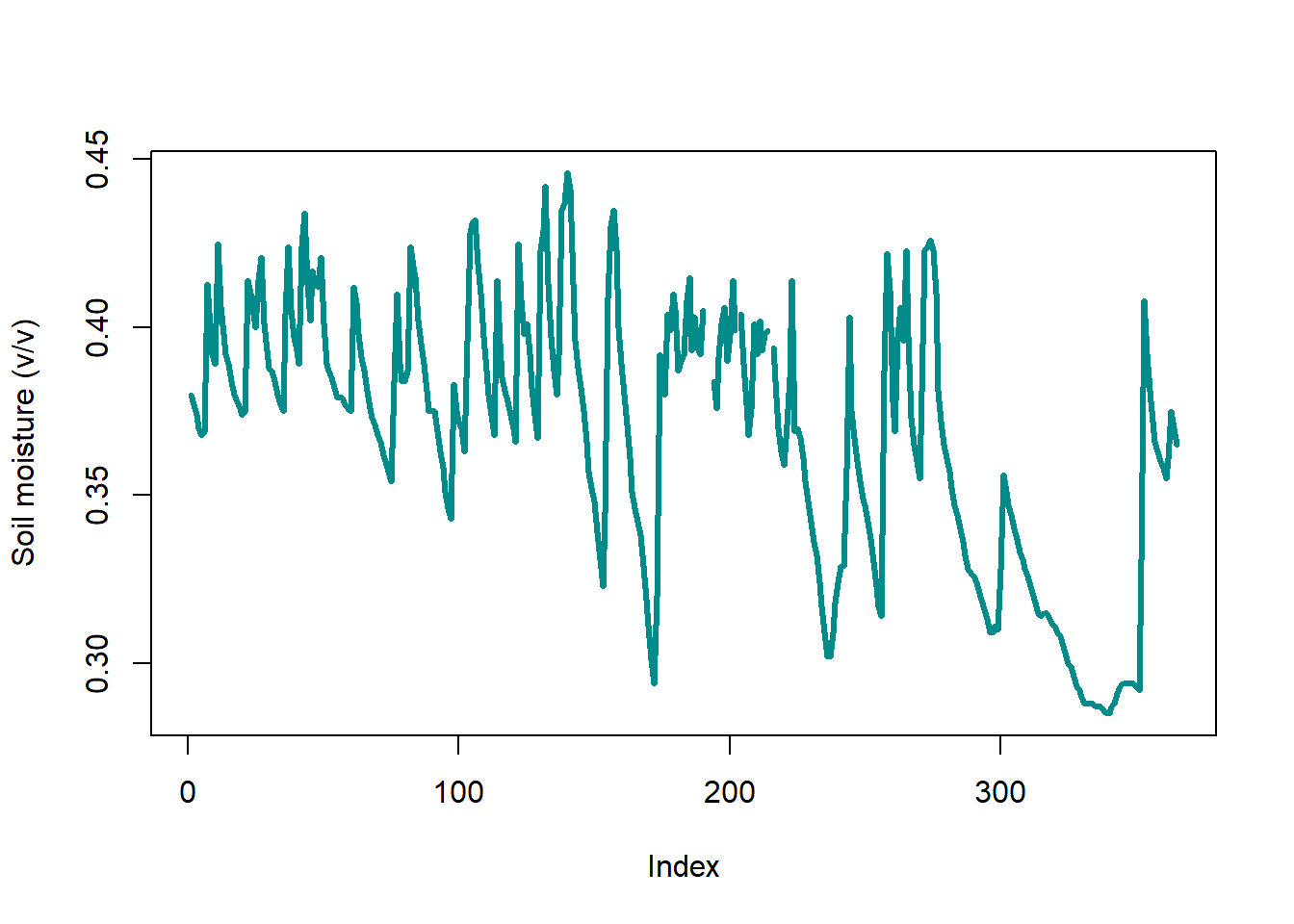
Notice the variables provided in the dataset. As an example, we can plots soil moisture data from a depth of 20 cm for this station for our reference:
# Sample plot for soil moisturex=CRNdat$SOIL_MOISTURE_20_DAILY# Plot time series and density distribution plot(x, type="l", ylab="Soil moisture (v/v)", col="cyan4", lwd=3)plot(density(na.omit(x)), main=" ", xlab="", col="cyan4", lwd=3)
(a) Time series of SM
(b) SM kernel density
Figure 12.1: Soil moisture values at the selected USCRN station
Taking examples of any two USCRN stations across contrasting hydroclimates, compare and contrast any two recorded variables using time series plots, probability density distribution histograms and scatter plots. Select any year of your liking for the analysis.
Select two seasons for each elected variable and demonstrate the seasonal variability in the records for summer (MAMJJA) and winter (SONDJF) seasons using any two types of multivariate plots.
12.3 Exercise #2
Use the raster files in SampleData-master/SMAPL4_rasters folder, and perform the tasks as listed below:
Task 1: Write a user-defined function to count the number of pixels within the range [0.3, 0.4] for 20211213. Use global to implement your function. Pass the specified range as an input argument to the function.
Task 2: Compared to 20211213, what is the percentage change in 20211215 for the pixels within the [0.3, 0.4] range?
Task 3: Make a multivariate plot (2 or more variables on the same axis) comparing the density distribution of soil moisture for 20211213 and 20211215?
12.4 Exercise #3
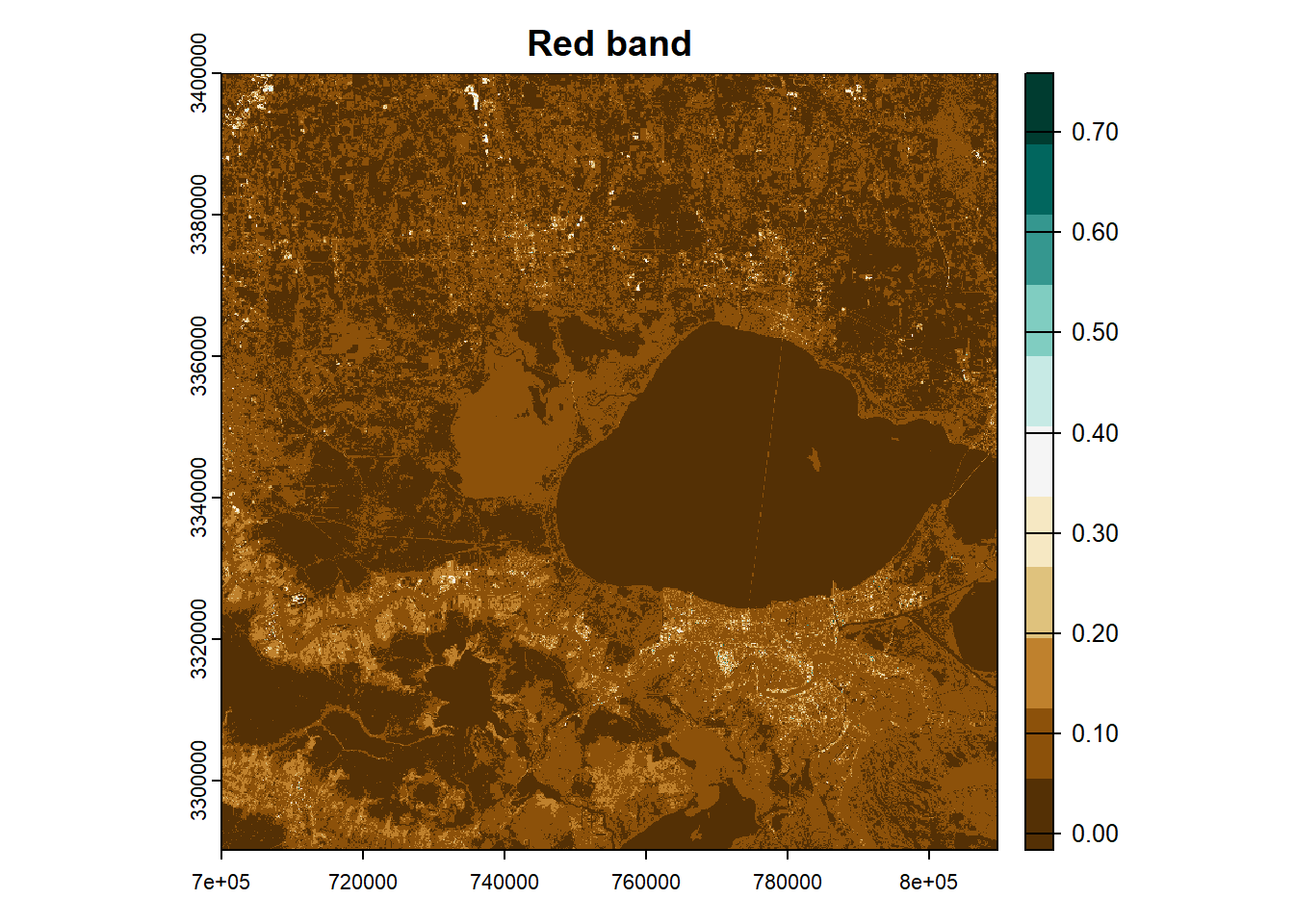
The Harmonized Landsat Sentinel-2 (HLS) project provides consistent multiband surface reflectance (SR) data from NASA/USGS Landsat 8 and Landsat 9 satellites (using Operational Land Imager, OLI) and Europe’s Copernicus Sentinel-2A and Sentinel-2B satellites (using Multi-Spectral Instrument, MSI). These measurements provide global land observations with a 2–3 days temporal frequency at 30-meter spatial resolution. Sample rasters for band 4 (Red) and band 5 (Near-Infrared) from this resource are provided at the following location in the sample data: “./SampleData-master/raster_files/landsat/”
For LANDSAT 8, the Normalized Difference Vegetation Index (a proxy for vegetation health) is calculated as:
Using the spectral band rasters provided above, complete the following objectives:
(10) Generate and plot NDVI raster for the areal domain. [HINT: Use multi-raster arithmetic from 4.1.2]
(10) Reproject the NDVI raster to the following projection: North American Datum 1983 (NAD83, refer to Sec 3.2.8 for help)
(10) Clamp the range of the NDVI to [-1,1]. [Hint: Checkout the flash card at the end of chapter 4 or try ?t erra::clamp]
(10) Plot the reprojected NDVI raster and add the following locations of interest to the map [Hint: Check out Sec 3.2.8]:
Location 1: Lon1=-90.6, Lat1= 30.4
Location 2:Lon2=-90, Lat2= 30.1
(10) Extract NDVI values for the two locations given above. [Hint look at the example for extract in 6.3.1]
(20) Crop the NDVI raster to the following extent and plot the cropped raster: [Xmin, Xmax, Ymin, Ymax]= [-90.5, -90.4, 30.05, 30.15]. [HINT: Create a vector using the extent and use it for cropping]
(30) Use NASA Earth Data Search (as shown in Section 6.2.6) to download Harmonized Landsat Sentinel-2 (HLS) surface reflectance for band 4 and 5 for any date and region of your choice. Repeat objectives 1 through 3 and plot the resultant NDVI raster.
12.5 Exercise #4
Imagine that a federal agency is interested in understanding the impacts of land conservation practices to improve carbon sequestration in the soil. The agency has selected two potential Carbon Sequestration Testbed (CST) sites across Louisiana. Using the observations of hydrometeorological, land practice, and vegetation datasets collected from these locations, the agency is interested in developing a physics-based ecohydrology model to mimic the interactions between soil, plants, and atmosphere at these test beds. This will help develop predictive models to estimate the effects of various management practices on the carbon sequestration potential in soil.
library(terra)library(mapview)# Import vector for Louisiana LAvct=vect(spData::us_states[spData::us_states$NAME=="Louisiana",])# Spatial attributes of the test polygonslon =c(-89.9, -90.2, -90.2,-93,-92.8, -93.1)lat =c(30.8, 30.8, 30.5,32, 32.2, 32.4)id=c(1, 1, 1, 2, 2, 2)# Combine attributes by columnslonlat =cbind(id, lon, lat)# Create polygons using the point locations as vertices#~~~ CRS of the LA vect is assigned to the new vectorCSTpoly =vect(lonlat, type="polygons",crs=crs(LAvct))# Add polygon id to the vector geometryCSTpoly$CST=c(1,2)# Plot map of Louisiana with overlaying CST polygonsmapview(LAvct, alpha.regions =0.1) +mapview(CSTpoly, zcol ="CST", col.regions =c("blue", "red"))
To develop these ecohydrology models, the agency needs your assistance in collecting high-resolution soil texture dataset for the Louisiana CSTs. You know from Ch 6 that soil texture data is available through POLARIS at [30m X 30m] spatial resolution for 6 soil depths (0-5 cm, 5-15 cm, 15-30 cm, 30-60 cm, 60-100 cm and 100-200 cm. So, for this exercise, you will generate the maps of mean percent clay content for 0-100 cm soil profile for the two CSTs by taking the arithmetic average of the clay percent in each layer between 0-100 cm depth. Access the mean clay content data from: http://hydrology.cee.duke.edu/POLARIS/PROPERTIES/v1.0/clay/mean/.
For each CST, follow the following steps:
(10) Use R code to download the .tif files for the areal domain encompassing the polygon for 0-5 cm soil profile.
(15) Combine the rasters using the mosaic function.
(15) Crop and mask the mosaic raster to the polygon extent and shape.
(20) Repeat for other soil profiles.
(20) Take cell-wise arithmetic average of the mean soil percentage for the layers.
(10) Plot the raster (mean soil percentage for 0-100 cm) for the CST.
(10) Export the raster.
12.6 Exercise #5
Soil moisture is an important hydrological variable with strong linkages to crop health and yield. Satellites such as NASA’s SMAP and ESA’s SMOS provide soil moisture information for the surface profile (0-5 cm). However, temporal variability in the surface soil moisture gets attenuated and dampened as water infiltrates through the soil layers. This is followed by evapotranspirative losses to the atmosphere from the rootzone. The time delay in surface soil moisture and evapotranspiration variability indicates several critical aspects of ecosystem functioning, terrestrial water and energy balance and soil hydraulic processes.
In this exercise, we will simulate the attenuation and dampening effect on the surface soil moisture using a moving average filter and study how increasing smoothing of surface soil moisture correlates with the variability in evapotranspiration. We will use simulated gridded surface soil moisture and evapotranspiration from VIC land surface model for the year 2011.
Download CONUS-wide daily simulated soil moisture (soilmoist.2011.nc) and evapotranspiration (et.2011.nc) for the year 2011 from NOAA-PSL’s servers. using the following file location:
Import the downloaded netCDFs to workspace as spatRasters. Print the time stamp and variable names of the two spatRasters using terra::time() and terra::names() functions. You will notice that et.2011.nc has one raster layer for each day. soilmoist.2011.nc contains three raster layers (one for each soil profile level) per day.
Create a new multilayer spatRaster for raster layers for soil profile level 1. (Hint: using substr() on the layer names() from soilmoist.2011.nc, subset the layers with lev= “1” in their name)
Create a polygon with with extent: xmin=255, xmax=265, ymin=40, ymax=48.
a) Plot a map of level 1 soil moisture for day 10 and overlay the polygon on the map.
b) Crop evapotranspiration and soil moisture spatRasters to the spatial polygon.
c) Plot the raster layers for day 10 from the cropped evapotranspiration and soil moisture SpatRasters.
If smTS is the soil moisture time series, and Tagg is the time-period of moving average, the function generates a right aligned rolling mean (moving average) of the time series. NA is used as fill values for the first Tagg-1 cells of the output.
Create and report a custom function for applying the moving average on a time series with the following components:
a) Two input arguments:
i) minSamp (minimum number of samples in a time series)
ii) Tagg (time period of aggregation)
b) Error exception using trycatch, where the function returns NA series for the pixel where error occurs.
For a point of interest at Lon=260, Lat=45:
Extract a sample time series from level 1 soil moisture
Apply the custom function made in the previous step to the sample time series.
Generate soil moisture moving average for the selected location with for four Tagg values, 7, 15, 30 and 45 days. Keep minSamp fixed at 100.
Plot the extracted level 1 soil moisture time series for the point of interest. Overlay aggregated time series at Tagg=7, 15, 30, 45 on the same x-axis. Comment on the relationship between Tagg and time series smoothing.
Apply the custom moving average function in parallel on each grid of the cropped multilayer soil moisture SpatRaster (from step 4) with Tagg=7, 15, 30, 45. Keep minSamp fixed at 100. Use all-but-one available system cores for parallel computing.
If x and y are two time series, then the following operation gives the Pearson’s correlation between the two datasets:
cor(x, y, use = "pairwise.complete.obs")
Using a custom function, calculate cell-wise correlation between evapotranspiration and moving averaged level 1 soil moisture for Tagg=7, 15, 30 and 45. (Hint: ?terra::xapp)
Create a multilayer raster by concatenating the output rasters from Step 8.
Plot the multilayer rasters of grid-wise correlation between evapotranspiration and level 1 soil moisture with Tagg =7, 15, 30 and 45. Fix legend range as (0,1).
Using global() function on the concatenated rasters, calculate and report the layer-wise median correlation between evapotranspiration and moving averaged level 1 soil moisture for the areal domain.