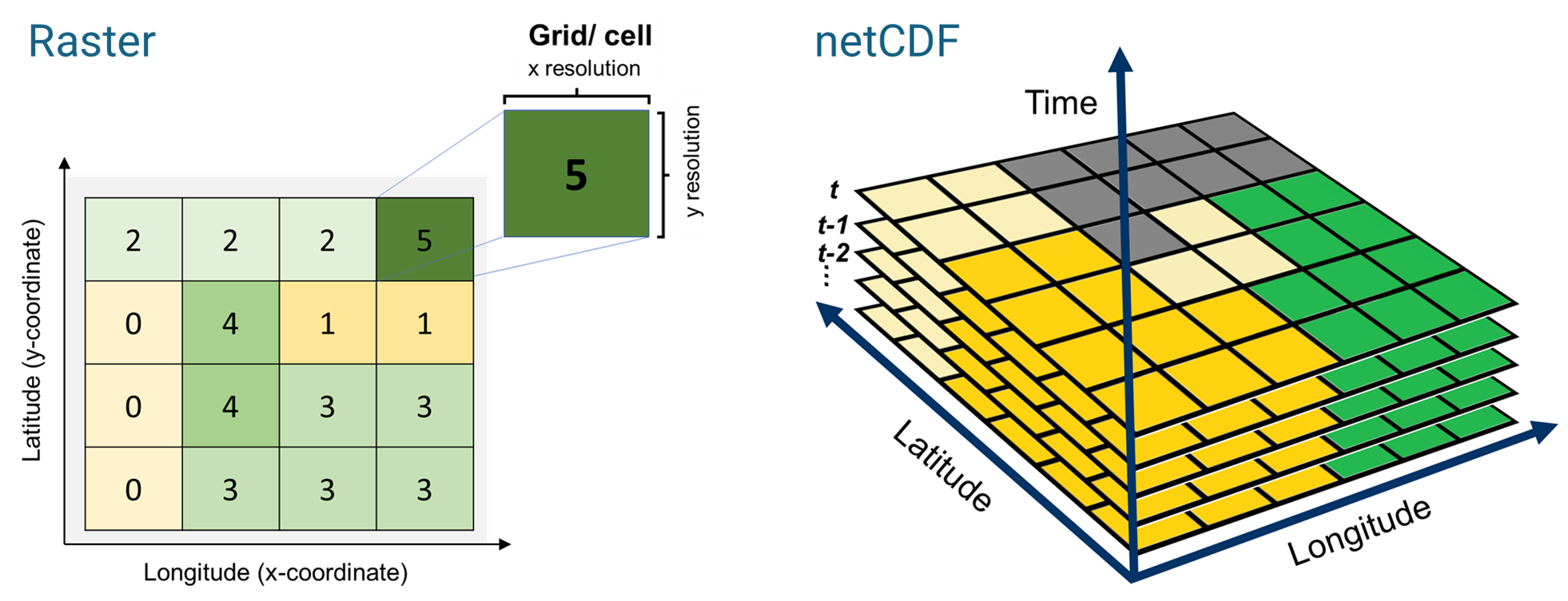
Raster and netCDF are two popular formats used for gridded climate data dissemination and archiving.
We are all too familiar with the raster format (pixelated, georeferenced data) from the previous chapters. NetCDF (Network Common Data Form), is a common data type for multi-layered, structured, gridded dataset. NetCDF is a machine-independent data format and is a community standard for sharing scientific data. A netCDF has certain features which makes it suitable for complex scientific data archiving and sharing, namely,
Self-Describing. A netCDF file includes information about the data it contains.
Portable. A netCDF file can be accessed by computers with different ways of storing integers, characters, and floating-point numbers.
Scalable. A small subset of a large dataset may be accessed efficiently.
Appendable. Data may be appended to a properly structured netCDF file without copying the dataset or redefining its structure.
Shareable. One writer and multiple readers may simultaneously access the same netCDF file.
Archivable. Access to all earlier forms of netCDF data will be supported by current and future versions of the software.
Two widely used formats for gridded climate data storage and dissemination: (Left) Raster and (Right) netCDF
Several open-source plaforms and agencies provide open access to a multitude of gridded land and climate datasets generated using satellites and land-surface/ climate models. In the following sections, we will familiarize ourselves with some of these resources.
6.2 Open-Data Platforms
6.2.1 Climate Data from NOAA Physical Sciences Lab
A snapshot of NOAA’s Physical Sciences Lab’s portal for gridded climate data access
This website provides several land and climate variables such as: CPC Global Unified Gauge-Based Analysis of Daily Precipitation, CPC Global Temperature, NCEP/NCAR Reanalysis, Livneh daily CONUS near-surface gridded meteorological and derived hydrometeorological data.
6.2.2 DAYMET: Daily Gridded Weather and Climate Data for North America [1 km x 1 km]
Data information: Refer to the User Guide provided with each dataset.
Daymet Webpage for Gridded Climate/ Weather Data Access
Daymet provides long-term, continuous, gridded estimates of daily weather and climatology variables at 1 km grid resolution for North America. The dataset is available in several forms, including monthly and annual climate summaries, in addition to the daily and/or sub-daily climate forcings:
FTP portal for NOAA’s Climate Prediction Center (CPC) data access
Includes several variables including (but not limited to):
Climate Prediction Center (CPC) Morphing Technique (MORPH) to form a global, high resolution precipitation analysis
Joint Agricultural Weather Facility (JAWF)
Grid Analysis and Display System (GRADS): Global precipitation monitoring and forecasts, Tmax, Tmin
Input variables for US Drought Monitor (USDM)
6.2.6 Soil Texture for CONUS [30 m x 30 m]
Probabilistic Remapping of SSURGO (POLARIS) is a database of 30-m probabilistic soil property maps over the Contiguous United States (CONUS) generated by removing artificial discontinuities in Soil Survey Geographic (SSURGO) database. using an artificial intelligence algorithm (Chaney et al. 2016, 2019). Estimates provided by POLARIS include soil texture, organic matter, pH, saturated hydraulic conductivity, Brooks-Corey and Van Genuchten water retention curve parameters, bulk density, and saturated water content for six profile depths, namely, 0-5 cm, 5-15 cm, 15-30 cm, 30-60 cm, 60-100 cm, 100-200 cm.
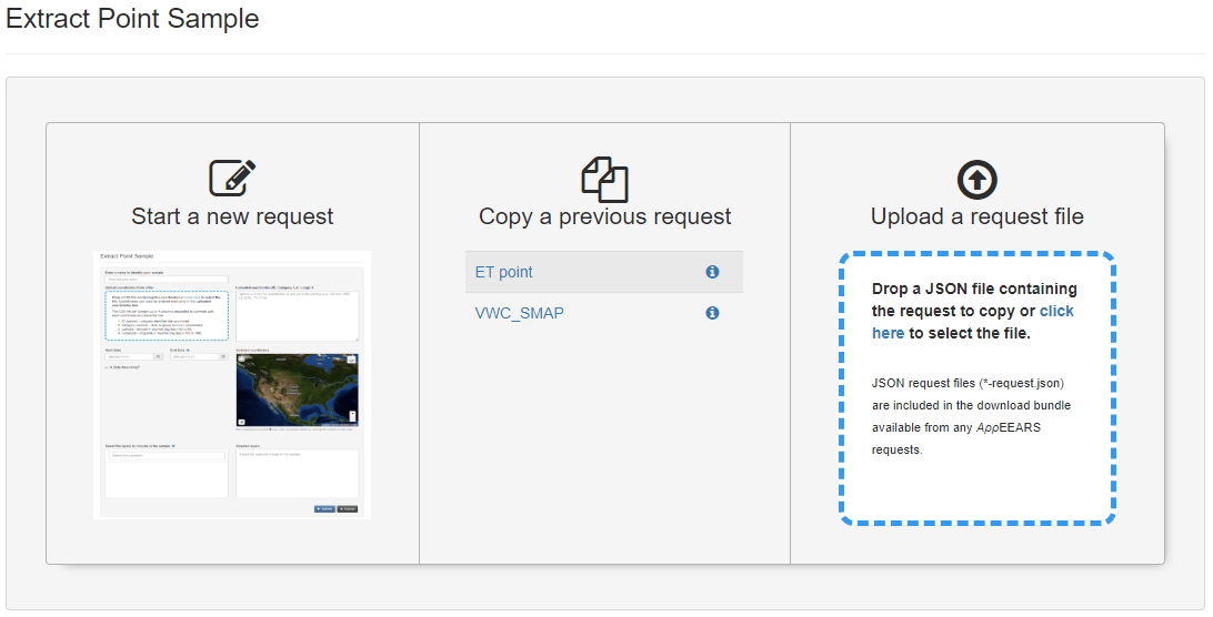
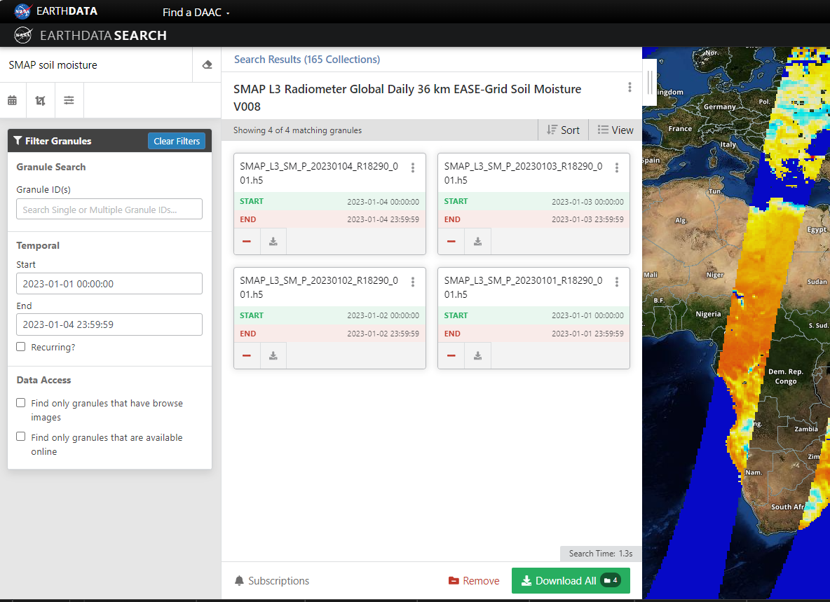
NASA Earth Data provides customization options for bulk data download. Lets say we are interested in downloading global SMAP Level 3 soil moisture. We start by selecting the product, and specify start/ end date as needed.
Search for the product, click “Download All”. You will be taken to a log-in page.
After logging in, Click “Edit Options”-> “Customize” and select options as needed. Click “Done”.
Click “Download Data”
A “Download Status” page will appear. Click on the “.html” link.
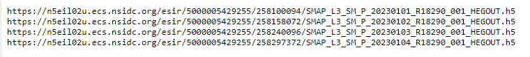
Several download options will available. For bulk download, click the link under “Retrieve list of files as a text listing (no html)”
You will be able to see the active download links.
Copy and Paste these links in any internet download manager (my favorite in Chrono for Google Chrome), Select output location (typically an external hard drive) and let the download begin.
6.3 Programmatic Data Acquisition
In the HTTP, FTP or HTP links provided before, one can download a file by clicking on the individual hyperlink. Alternatively, we can use download.file function to download the file programmatically in R. This help us by opening the path to automate download and processing of multiple files with minimal supervision.
6.3.1 Downloading Raster files
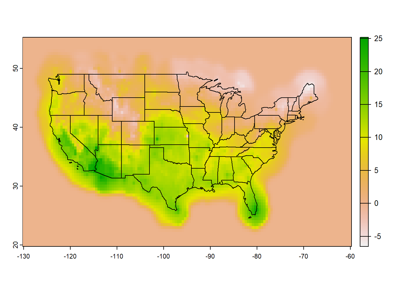
Let us take an example of us_tmax data available at: https://ftp.cpc.ncep.noaa.gov/GIS/GRADS_GIS/GeoTIFF/TEMP/us_tmax/
Right-click on the raster file for 20240218, and copy the file path. We will then use this link to access the files programmatically using Client URL, or cURL - a utility for transferring data between systems. We will download the raster using download.file to local disk, and saved with a uder-defined name tmax_20240218.tif.
# Copied path of the rasterdata_path <-"https://ftp.cpc.ncep.noaa.gov/GIS/GRADS_GIS/GeoTIFF/TEMP/us_tmax/us.tmax_nohads_ll_20240218_float.tif"# Download the raster using download.file, assign the name tmax_20240218.tif to the downloaded download.file(url = data_path, method="curl",destfile ="tmax_20240218.tif") # Plot downloaded filelibrary(terra)tempRas=rast("tmax_20240218.tif") # Import raster to the environment usSHP=terra::vect(spData::us_states) # Shapefile for CONUSplot(tempRas)plot(usSHP, add=TRUE)
Now that we have the tmax_20240218 raster, let us extract the values for certain selected locations: s
# Import sample locations from contrasting hydroclimatelibrary(readxl)loc=read_excel("./SampleData-master/location_points.xlsx")print(loc)
# A tibble: 3 × 4
  Aridity   State     Longitude Latitude
  <chr>     <chr>         <dbl>    <dbl>
1 Humid     Louisiana     -92.7     34.3
2 Arid      Nevada       -116.      38.7
3 Semi-arid Kansas        -99.8     38.8
# Value of the lat & lon of the locationslatlon=loc[,3:4] print(latlon)
# A tibble: 3 × 2
  Longitude Latitude
      <dbl>    <dbl>
1     -92.7     34.3
2    -116.      38.7
3     -99.8     38.8
# Extract time series using "terra::extract"loc_temp=terra::extract(tempRas, latlon, #2-column matrix or data.frame with lat-longmethod='bilinear') # Use bilinear interpolation (or ngb) optionprint(loc_temp)
library(spData)# Note the spatial extent of Louisiana State. We need corresponding raster filesext(spData::us_states[spData::us_states$NAME=="Louisiana",]) # ext function gives extent of the rast/vect object
pth1="http://hydrology.cee.duke.edu/POLARIS/PROPERTIES/v1.0/clay/mean/0_5/lat3031_lon-91-90.tif"# Download the raster using download.filedownload.file(url = pth1, method="curl",destfile ="lat3031_lon-90-89.tif") # Import the downloaded raster to workspacer1=rast("lat3031_lon-90-89.tif")# Fetch shapefile for Louisiana from spData packageLAvct=vect(spData::us_states[spData::us_states$NAME=="Louisiana",])# Plot downloaded raster against the map of Louisiana. Note that the raster fits 1x1 gridplot(LAvct, col="gray90")plot(r1, range=c(0,100), add=TRUE)grid()
# Crop raster to smaller region of interest for easy visualization#~~~ We will crop raster to a user-defined extentr1crp=crop(r1, ext(c(-91,-90.8,30,30.2))) # Explore a smaller subset of the dataset#~~~ Can you identify the Mississipi flood-plain using the clay percentage? library(mapview)mapview(r1crp, # Raster to be plottedat=c(0,10,20,30,40,50,60,75), # Legend breaksmap.types="Esri.WorldImagery", # Select background map main="Clay % (0-5 cm profile)") # Plot title
We note that the raster files in POLARIS are available for a 1x1 areal domain. For an analysis for a large spatial extent, multiple smaller rasters can be “stitched” together to generate a larger mosaic of rasters. We will use the terra::mosaic function to generate a mosaic of several smaller rasters of percentage clay content in 0-5 cm soil profile in Southeastern Louisiana. This function requires the user to specify the summary function (“sum”, “mean”, “median”, “min”, or “max”) to be applied on the overlapping pixels from 2 or more rasters. Let us download some more rasters from POLARIS and mosaic them together.
“Beware of the dog” mosaic (Pompeii, Casa di Orfeo) is made of several constituent pieces.
# Links to soil texture rasters pth2="http://hydrology.cee.duke.edu/POLARIS/PROPERTIES/v1.0/clay/mean/0_5/lat2930_lon-91-90.tif"pth3="http://hydrology.cee.duke.edu/POLARIS/PROPERTIES/v1.0/clay/mean/0_5/lat3031_lon-90-89.tif"pth4="http://hydrology.cee.duke.edu/POLARIS/PROPERTIES/v1.0/clay/mean/0_5/lat3031_lon-92-91.tif"# Download the raster using download.file functiondownload.file(url = pth2, method="curl",destfile ="r2.tif") download.file(url = pth3, method="curl",destfile ="r3.tif")download.file(url = pth4, method="curl",destfile ="r4.tif") # Import downloaded files to workspacer2=rast("r2.tif")r3=rast("r3.tif")r4=rast("r4.tif")# DIY: Plot the downloaded raster against the map of Louisiana# plot(LAvct)# plot(r1, range=c(0,100), add=TRUE)# plot(r2, range=c(0,100), add=TRUE, legend=FALSE)# plot(r3, range=c(0,100), add=TRUE, legend=FALSE)# plot(r4, range=c(0,100), add=TRUE, legend=FALSE)# Raster mosaicr_mos=mosaic(r1,r2,r3,r4, fun="mean")# Plot raster mossaicplot(LAvct, main="Clay % [0-5 cm depth]",axes=FALSE, col="gray90")plot(r_mos, range=c(0,100), add=TRUE)plot(LAvct, add=TRUE)grid()
For easy post processing access, its a good practice to save the processed dataset on disc as either a raster or netCDF.
# Export raster to discterra::writeRaster(r_mos, "clayPct.tif",overwrite=TRUE) # Overwrite if the file already exists?# Or export as netCDFterra::writeCDF(r_mos, "clayPct.nc", overwrite=TRUE) # Overwrite if the file already exists?# Optional: Add more information to the exported netCDF# terra::writeCDF(r_mos, # SpatRaster to export# "clayPct.nc", # Output filename# varname="clayPCT", # Short name of the variable# unit="%", # Variable units# longname="Clay Percentage, 0-5 cm, POLARIS", # Long name of the variable# zname='[-]') # Z-var name (None, since we export a single layer)
6.3.3 Downloading netCDF
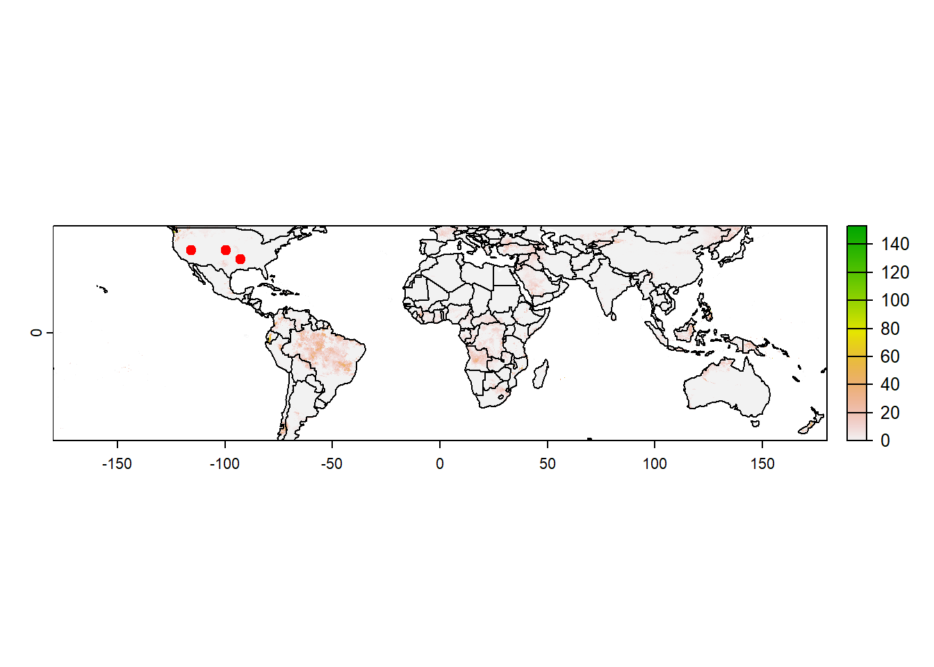
We will now download a netCDF of global daily precipitation for the year 2023 from CHIRPS, accessible through the link: https://data.chc.ucsb.edu/products/CHIRPS-2.0/global_daily/netcdf/p05/chirps-v2.0.2023.days_p05.nc
# Copied path of the rasterdata_path <-"https://data.chc.ucsb.edu/products/CHIRPS-2.0/global_daily/netcdf/p05/chirps-v2.0.2023.days_p05.nc"# Download the raster using download.file, assign the name "daily_pcp_2023.nc" to the downloaded if (file.exists("daily_pcp_2023.nc")==FALSE){download.file(url = data_path, method="curl",destfile ="daily_pcp_2023.nc") }# Plot downloaded filelibrary(terra)pcp=rast("daily_pcp_2023.nc") # Import raster to the environment print(pcp) # Notice the attributes (esp. nlyr, i.e. number of layers, unit and time)
worldSHP=terra::vect(spData::world) # Shapefile for CONUS# Plot data for a specific layerplot(pcp[[100]]) # Same as pcp[[which(time(pcp)=="2023-04-10")]]plot(worldSHP, add=TRUE)points(latlon, pch=19, col="red")
Chaney, Nathaniel W, Budiman Minasny, Jonathan D Herman, Travis W Nauman, Colby W Brungard, Cristine LS Morgan, Alexander B McBratney, Eric F Wood, and Yohannes Yimam. 2019. “POLARIS Soil Properties: 30-m Probabilistic Maps of Soil Properties over the Contiguous United States.”Water Resources Research 55 (4): 2916–38.
Chaney, Nathaniel W, Eric F Wood, Alexander B McBratney, Jonathan W Hempel, Travis W Nauman, Colby W Brungard, and Nathan P Odgers. 2016. “POLARIS: A 30-Meter Probabilistic Soil Series Map of the Contiguous United States.”Geoderma 274: 54–67.