While soil moisture’s centrality in precipitation partitioning into groundwater recharge and surface runoff is widely recognized, often the criticality of the surface and rootzone connectivity is overlooked. You might have read about incessant rainfall after a dry and hot period often generates flash floods. Why? Because the surface profile might get hydrophobic, and hence, hydrologically decoupled from the rootzone under intense heat. So, a larger fraction of the incoming rain contributes to overland runoff instead of infiltrating to the rootzone, and contributing to the groundwater recharge. So, hydrologic connectivity between surface and the rootzone profile directly affects critical ecohydrological processes such as groundwater recharge, surface runoff generation, and the overall water availability for ecosystem sustenance. Needless to say, knowing how moisture moves from the surface to the rootzone can improved water management to ensure sustained and adequate moisture to the crops, while preventing over-irrigation. Accurate data on both surface and rootzone soil moisture also helps in improving weather forecasts and seasonal-scale climate forecasts, thereby helping to predict and manage hydrologic extremes such as droughts and floods.
In this chapter, we will explore the hydrologic relationship between surface and the rootzone profile, and methods to simulate these processes.
10.1.1 Exploratory Data Analysis for the Sample Station
We will use in situ (ground) measurements from a sample station to discuss various attributes of moisture dynamics in the field and learn the relationship between moisture and thermal fluxes of surface and deeper profiles. For this purpose, we will use a station from U.S. Climate Reference Network (USCRN) at Stillwater, Oklahoma. USCRN is instrumented to measure meteorological information such as temperature, precipitation, wind speed, along with other relevant hydrologic variables such as soil moisture and temperature at 5-, 10-, 20-, 50- and 100 cm depths at sub-hourly, daily and monthly time scales. For our example, we will use daily dataset for 2021.
# Download in situ data files for 2021 from GITHUB repositiry utils::download.file("https://github.com/Vinit-Sehgal/SampleData/blob/master/CRN_data/CRND0103-2021-OK_Stillwater_2_W.txt?raw=true",destfile ="CRND0103-2021-OK_Stillwater_2_W.txt", mode="wb", #wb is write binarymethod ='auto', quiet=FALSE)utils::download.file("https://github.com/Vinit-Sehgal/SampleData/blob/master/CRN_data/HEADERS.txt?raw=true",destfile ="headers.txt", mode="wb", #wb is write binarymethod ='auto', quiet=FALSE)CRNdat =read.csv("CRND0103-2021-OK_Stillwater_2_W.txt", header=FALSE,sep="")headers =read.csv("headers.txt", header=FALSE,sep="")# OR Direct download from NCEI servers (might not work during server downtime)#CRNdat = read.csv(url("https://www.ncei.noaa.gov/pub/data/uscrn/products/daily01/2021/CRND0103-2021-OK_Stillwater_2_W.txt"), header=FALSE,sep="")# Data headers#headers=read.csv(url("https://www.ncei.noaa.gov/pub/data/uscrn/products/daily01/headers.txt"), header=FALSE,sep="")# Column names as headers from the text filecolnames(CRNdat)=headers[2,1:ncol(CRNdat)]# Replace fill values with NACRNdat[CRNdat ==-9999]=NACRNdat[CRNdat ==-99]=NACRNdat[CRNdat ==999]=NA# View data samplelibrary(kableExtra)dataTable =kbl(head(CRNdat,6),full_width = F)kable_styling(dataTable,bootstrap_options =c("striped", "hover", "condensed", "responsive"))
WBANNO
LST_DATE
CRX_VN
LONGITUDE
LATITUDE
T_DAILY_MAX
T_DAILY_MIN
T_DAILY_MEAN
T_DAILY_AVG
P_DAILY_CALC
SOLARAD_DAILY
SUR_TEMP_DAILY_TYPE
SUR_TEMP_DAILY_MAX
SUR_TEMP_DAILY_MIN
SUR_TEMP_DAILY_AVG
RH_DAILY_MAX
RH_DAILY_MIN
RH_DAILY_AVG
SOIL_MOISTURE_5_DAILY
SOIL_MOISTURE_10_DAILY
SOIL_MOISTURE_20_DAILY
SOIL_MOISTURE_50_DAILY
SOIL_MOISTURE_100_DAILY
SOIL_TEMP_5_DAILY
SOIL_TEMP_10_DAILY
SOIL_TEMP_20_DAILY
SOIL_TEMP_50_DAILY
SOIL_TEMP_100_DAILY
53926
20210101
2.622
-97.09
36.12
2.1
0.2
1.2
0.8
23.0
3.51
C
1.0
-0.3
0.3
93.1
70.1
86.2
0.474
0.440
0.458
0.450
0.429
3.9
4.2
5.4
8.3
9.9
53926
20210102
2.622
-97.09
36.12
6.9
-2.5
2.2
1.8
0.0
7.02
C
9.9
-4.7
1.1
94.2
57.3
78.7
0.466
0.443
0.459
0.448
0.432
4.6
4.7
5.5
8.0
9.6
53926
20210103
2.622
-97.09
36.12
9.1
-3.7
2.7
1.3
0.0
10.56
C
12.9
-6.2
-0.2
94.2
56.4
83.5
0.436
0.440
0.460
0.449
0.429
4.2
4.7
5.5
7.8
9.4
53926
20210104
2.622
-97.09
36.12
14.7
-3.2
5.7
4.3
0.0
11.13
C
16.8
-6.0
2.0
94.0
46.2
76.4
0.423
0.428
0.461
0.450
0.430
4.6
5.0
5.6
7.6
9.2
53926
20210105
2.622
-97.09
36.12
16.2
-3.6
6.3
6.2
0.0
9.99
C
17.9
-6.5
3.9
94.0
22.0
59.5
0.412
0.417
0.463
0.453
0.431
4.8
5.2
5.7
7.6
9.1
53926
20210106
2.622
-97.09
36.12
9.6
4.8
7.2
7.5
0.3
1.03
C
11.4
4.3
7.1
92.1
45.8
66.7
0.395
0.412
0.459
0.450
0.431
6.2
6.1
6.2
7.6
9.1
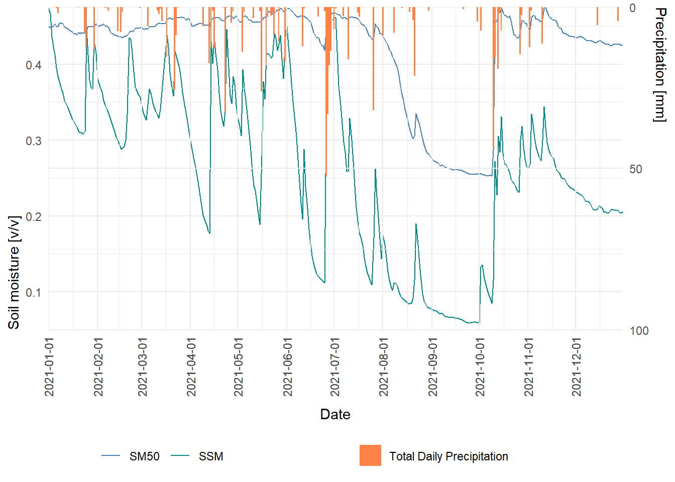
Let’s plot daily average soil moisture from 5 and and 50 cm depths, along with the corresponding daily total precipitation.
# Create Date array for the stationlibrary(zoo)library(cowplot)library(ggplot2)# Time (in days) datetime=as.Date(as.character(CRNdat$LST_DATE), format="%Y%m%d")# Surface soil moisture (in m3/m3) SSM=na.approx(CRNdat$SOIL_MOISTURE_5_DAILY,na.rm =FALSE) # Soil moisture at 50 cm depth (in m3/m3) SM50=na.approx(CRNdat$SOIL_MOISTURE_50_DAILY,na.rm =FALSE) # Precipitation (in mm) PCP=CRNdat$P_DAILY_CALC PCP[PCP<0]=0# Negative (flagged values are replaced by 0) PCP[is.na(PCP)]=0# NA values are replaced by 0)# Create a data frame of SM-PCP dataset for plotting df=data.frame(Date=datetime, PCP=PCP, SSM=SSM, SM50=SM50)# Plot for surface soil moisture p1 =ggplot(df) +geom_line(aes(Date, SSM, color ="SSM")) +geom_line(aes(Date, SM50, color ="SM50")) +scale_y_continuous(position ="left",limits =c(0.05,0.475),expand =c(0,0)) +scale_color_manual(values =c("steelblue", "cyan4")) +guides(x =guide_axis(angle =90)) +scale_x_date(date_breaks ="month",limits =c(datetime[1], datetime[365]),expand =c(0,0)) +labs(y ="Soil moisture [v/v]",x ="Date") +theme_minimal() +theme(axis.title.y.left =element_text(hjust =0),legend.position ="bottom",legend.justification =c(0.1, 0.5),legend.title =element_blank())# Plot for precipitation p2=ggplot(df) +geom_col(aes(Date, PCP, fill ="Total Daily Precipitation")) +scale_y_reverse(position ="right",limits =c(100,0),breaks =c(0,50,100),labels =c(0,50,100),expand =c(0,0)) +scale_x_date(date_breaks ="month",limits =c(datetime[1], datetime[365]),expand =c(0,0)) +scale_fill_manual(values =c("sienna1")) +guides(x =guide_axis(angle =90)) +labs(y ="Precipitation [mm]", x ="") +theme_minimal() +theme(axis.title.y.right =element_text(hjust =0),legend.position ="bottom",legend.justification =c(0.75, 0.5),legend.title =element_blank())aligned_plots = cowplot::align_plots(p1, p2, align ="hv", axis ="tblr")p3=ggdraw(aligned_plots[[1]]) +draw_plot(aligned_plots[[2]])print(p3)
We can notice that the temporal response of surface soil moisture to a precipitation varies significantly compared to that of the deeper profile. Surface soil moisture reacts almost immediately to precipitation. This layer, typically the top few centimeters, quickly absorbs rainfall, leading to a rapid increase in moisture content. Similarly, the surface, having exposed to atmospheric conditions, also dries out rapidly due to evaporation and plant water uptake. In contrast, soil moisture from the rootzone (typically up to about 1 meter) responds more slowly to precipitation as it relies on the infiltration of water from the surface layer. As infiltration delays moisture transfer to the rootzone profile. This results in a delayed but more gradual increase in rootzone moisture content. Similarly, rootzone also retains water longer. This ensures a more consistent and reliable source of water for plant growth and ecosystem stability. A similar behavior can also be seen in the temperature distribution within the soil profile. The difference in the temporal response of rootzone moisture and thermal fluxes vis-à-vis surface profile is essentially a natural manifestation of a low pass filter, where the high-frequency variations (rapid changes) in surface soil moisture or temperature are filtered out, leaving only the low-frequency variations (slower, more sustained changes) to affect the rootzone.
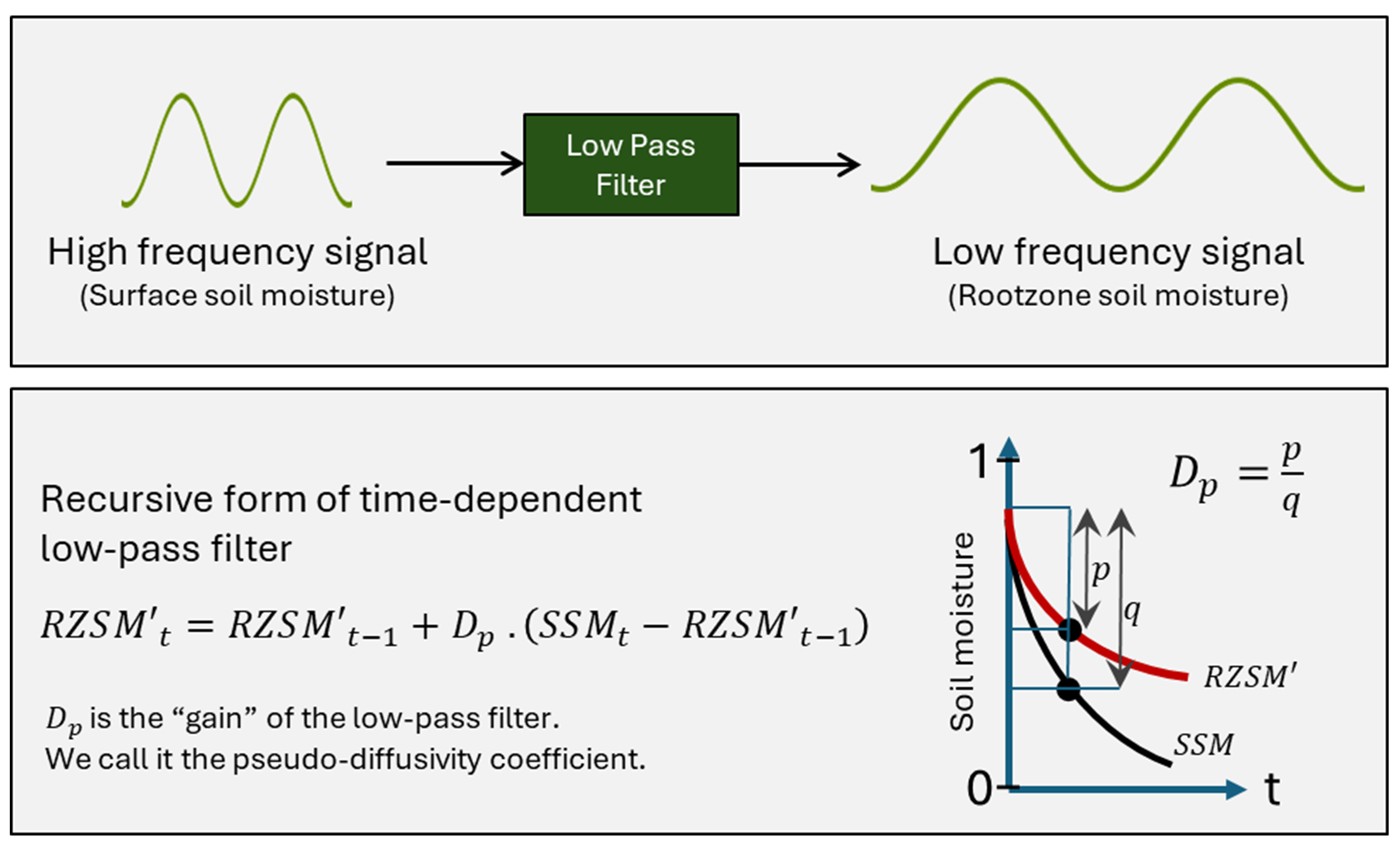
Figure 1: (Top) A schematic representation of low-pass filter effect on a time series. (Bottom) A reccursive form of low-pass filter on surface soil moisture.
# Profile depth versus soil temperatureTempdf=data.frame(T5=na.approx(CRNdat$SOIL_TEMP_5_DAILY,na.rm =FALSE), T10=na.approx(CRNdat$SOIL_TEMP_10_DAILY,na.rm =FALSE), T20=na.approx(CRNdat$SOIL_TEMP_20_DAILY,na.rm =FALSE), T50=na.approx(CRNdat$SOIL_TEMP_50_DAILY,na.rm =FALSE),T100=na.approx(CRNdat$SOIL_TEMP_100_DAILY,na.rm =FALSE))df=rbind(data.frame(Temp=Tempdf$T5, Depth=5,Date= datetime),data.frame(Temp=Tempdf$T10, Depth=10, Date=datetime),data.frame(Temp=Tempdf$T20, Depth=20,Date= datetime),data.frame(Temp=Tempdf$T50, Depth=50,Date=datetime),data.frame(Temp=Tempdf$T100, Depth=100, Date=datetime))ggplot(df, aes(x = Date, y = Depth)) +geom_contour_filled(aes(z = Temp), bins =6, stat ="contour_filled") +scale_fill_brewer(palette ="YlOrRd",direction =1) +labs(x ="Date", y ="Depth (cm)", fill ="Temperature (°C)") +theme_minimal() +scale_y_reverse()# Profile depth versus soil moistureSMpdf=data.frame(SM5=na.approx(CRNdat$SOIL_MOISTURE_5_DAILY,na.rm =FALSE), SM10=na.approx(CRNdat$SOIL_MOISTURE_10_DAILY,na.rm =FALSE), SM20=na.approx(CRNdat$SOIL_MOISTURE_20_DAILY,na.rm =FALSE), SM50=na.approx(CRNdat$SOIL_MOISTURE_50_DAILY,na.rm =FALSE),SM100=na.approx(CRNdat$SOIL_MOISTURE_100_DAILY,na.rm =FALSE))df=rbind(data.frame(SM=SMpdf$SM5, Depth=5,Date= datetime),data.frame(SM=SMpdf$SM10, Depth=10, Date=datetime),data.frame(SM=SMpdf$SM20, Depth=20,Date= datetime),data.frame(SM=SMpdf$SM50, Depth=50,Date=datetime),data.frame(SM=SMpdf$SM100, Depth=100, Date=datetime))ggplot(df, aes(x = Date, y = Depth)) +geom_contour_filled(aes(z = SM), bins =6, stat ="contour_filled") +scale_fill_brewer(palette ="YlGnBu") +labs(x ="Date", y ="Depth (cm)", fill ="Soil Moisture") +theme_minimal() +scale_y_reverse()
(a) Depth versus soil temperature
(b) Depth versus soil moisture
Figure 10.1: Soil temperature and moisture response with profile depth
Note
A low-pass filter is a general name for the type of operations used to smooth out a time series by removing high-frequency fluctuations, leaving behind the underlying trend or low-frequency components. You may be more familiar with moving average smoothing, which calculates the average of a fixed number of consecutive data points, effectively smoothing out short-term fluctuations. Hence, moving average is also a low-pass filter.
10.2 Simulating Low-pass Filtering of Meteorological Perturbations Through Soil Profile
Under hydrologic equilibrium, the analytical solution of the 1-dimensional vertical water balance (differential) equation can be approximated using the relationship between the temporal changes in the rootzone soil moisture (RZSM) and the difference in SSM vis-à-vis the antecedent rootzone conditions (Wagner et al., 1999, Albergel et al., 2008, Manfreda et al., 2014). A simple recursive exponential low-pass filter to simulate the 1-dimensional first-order infinite-impulse response of RZSM to temporal variability in SSM is given as follows:
where, \(t \ge1\); when \(t=1\), \(RZSM_{t=0}^{'}=SSM_{t=0}\).
\(RZSM_{t}^{'}\) is the temporally smoothed (filtered) SSM at time \(t\) .
Parameter \(D_p\) is the exponential filter smoothing factor of the soil profile \([-]\), also called the pseudo-diffusivity coefficient; \(D_p\) ∈ [0,1]. It represents the effective influence of various bio-geo-physical controls such as vegetation, topography, hydroclimatology and pedological characteristics (soil profile thickness, effective soil hydraulic characteristics, etc.) on vertical fluxes between the soil surface and the rootzone.
Eq. 1 provides a first-order approximation of the infinite-impulse response of RZSM to temporal variability in SSM as \(RZSM^{'}\), and yields the exponential weighted average of the antecedent observations using weights proportional to the terms of the geometric progression: \(1, (1-D_p), (1-D_p)^2, ….(1-D_p)^n\), \(-\) the discrete form of an exponential function (Hunter, 1986; Perry, 2010). This method makes two key assumption:
The lateral moisture flux to/from the rootzone is negligible, and,
The groundwater table is significantly deeper than the rootzone depth.
10.2.1 Origins of Low-pass Filter Relationship in Vertical Soil Fluxes
The origins of the low-pass filter effect of soil profile on surface variability in soil moisture can be traced to the original equations for vertical flux of water int he unsaturated soil profile. We recall the Diffusivity version of Richard’s equation as follows:
where, \(D\) and \(K\) are the hydraulic diffusivity and conductivity of the soil profile, and are a function of the water content of the soil profile, \(z\) is the height above the bottom of the soil profile and \(\theta\) is the soil moisture content. The right hand side of this equation contains two terms, where \(\partial/\partial z (D(\theta)\partial/\partial z)\) accounts for the flux due to the suction gradient in the profile, while \(\partial K(\theta)/\partial z\) pertains to the role of gravity in the vertical flow of water. Given the equivalent suction exerted by the atmosphere is several order of magnitude compare to the gravitational head gradient, we can simplify the preceeding equation as:
First integral of this equation can be written as: \[
\frac{d\theta}{dt}=D(\theta)\frac{d\theta}{dz}+C
\tag{10.4}\] where, \(C\) is the constant of integration. Since there is no flow at the bottom boundary of the soil profile, \(d\theta/dz=0\) . Hence, \(C=0\). Writing the preceding equation in discrete form, we get:
As the soil reaches the second phase of drying, it enters a phase where the rate of soil drydown is slow, and the rate of loss of water from all depths can be assumed to be the same. Simplifying the previous equation for a simple 2-layer representation of soil profile, with \(SSM\) and \(RZSM\) representing the surface and rootzone soil moisture respectively, we can write Eq. 5 as: \[
RZSM_t-RZSM_{t-1}= D(RZSM) \times (SSM_{t}-RZSM_{t-1})
\] or, \[
RZSM_t=RZSM_{t-1}+ D(RZSM) \times (SSM_{t}-RZSM_{t-1})
\tag{10.6}\]
However, such coarse discretization of the soil profile may not account for the different initial values of true surface and rootzone soil moisture, and may lead to a systematic bias in the estimated values of \(RZSM\) using the low-pass filter approach compared to the observations. This equation becomes analogous to the exponential infinite impulse response low-pass filter equation provided in Eq. 1 earlier. The filtered surface soil moisture i.e. \(RZSM'\) can be related to the true rootzone SM through a linear transformation as: \(RZSM= C \times RZSM^{'}+\epsilon\), where, \(C\) is the ratio of the dynamic range of \(RZSM\) and \(RZSM'\) as follows: \[
C= \frac {\max(RZSM)-min(RZSM)} {max(RZSM^{'})-min(RZSM^{'})}
\tag{10.7}\] and, \[
\epsilon=min(RZSM)-C \times min(RZSM^{'})
\tag{10.8}\]
Note
Hydraulic diffusivity (or pseudo-diffusivity) is a function of the hydrologic state of the rootzone. However, since the true form of the relationship between \(D-RZSM\) or \(Dp-RZSM^{'}\) is not known in the field, the value of \(D\) and \(D_p\) is often assumed to be constant for simplicity.
10.2.2 Propagation of Drying Front in the Soil Profile
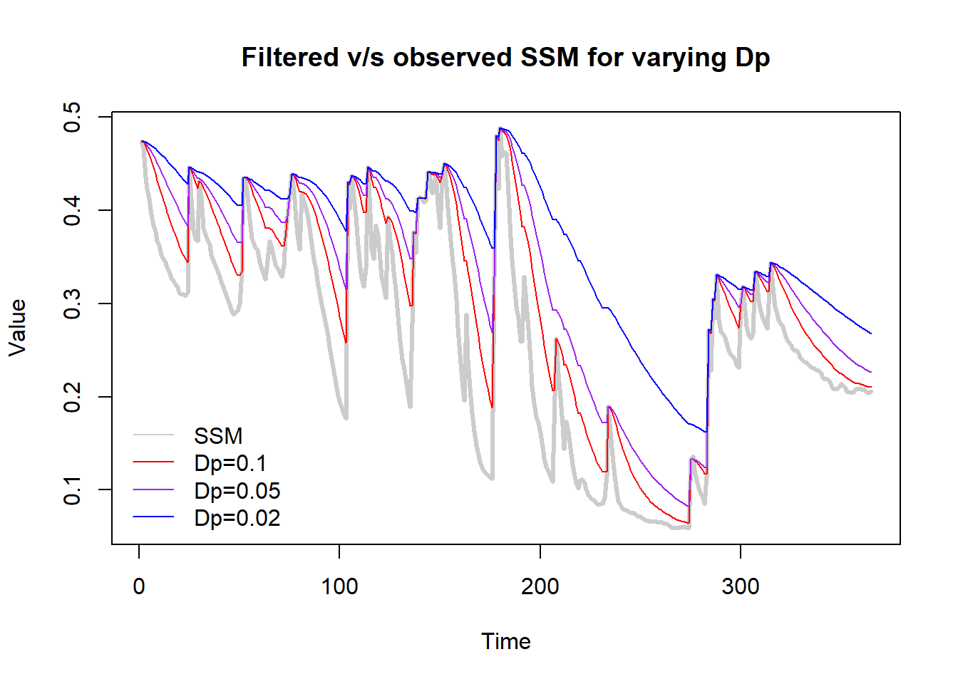
We will demonstrate the application of the low-pass filter discussed above to capture the propagation of drying front from the surface to the deeper profiles at the test site.The function lp_filt takes the SSM as input, apply a low-pass infinite impulse response filter on the time series for the user-specified \(Dp\), and returns the filtered SSM (SSMf). In contrast, the wetting front propagation is represented as a pulse which is passed down to the filtered soil moisture in the preceding time step.This assumption is reasonably valid at the daily time scale at which this example is applied.
# Function for implementing LP filter on surface soil moisturelp_filt=function(SSM, Dp){# PARAMETERS---# SSM= Surface soil moisture# Dp= Pseudo-diffusivity coefficient SSMf=c() # Empty array to store filtered SSM buffer=0.01*(max(SSM)-min(SSM)) # To decrease sensitivity to noise in sensor readings (1% of SSM range)# Apply recursive filter SSMf[1]=SSM[1] # Initialize the seriesfor (t in2:length(SSM)) SSMf[t]=ifelse(SSM[t] > (SSM[t-1]+buffer),max(SSM[t], SSMf[t-1]),SSMf[t-1]+Dp*(SSM[t]-SSMf[t-1]))return(SSMf) }# Filtered surface soil moisture with varying values of DpSSM=SMpdf$SM5 # Surface soil moistureSSMf_1=lp_filt(SSM, Dp=0.1)SSMf_05=lp_filt(SSM, Dp=0.05)SSMf_02=lp_filt(SSM, Dp=0.02)# Plot surface soil moisture with filtered time seriesplot(SSM, type="l", col="gray80", lwd=3, ylab="Value", xlab="Time", main="Filtered v/s observed SSM for varying Dp")lines(SSMf_1, col="red")lines(SSMf_05, col="purple")lines(SSMf_02, col="blue")legend(x ="bottomleft", legend =c("SSM","Dp=0.1", "Dp=0.05", "Dp=0.02"), lty =c(1,1,1,1), col =c("gray80","red","purple","blue"), lwd =1, bty ="n")
Note
We observe that the low-pass filter is only applied during the drydown phase of the surface soil moisture moisture. As the value of \(D_p\) decreases, the rate of drydown in \(SM^{'}\) decreases due to the increase in the e-folding time of the exponential filter applied.
Multi-depth soil moisture records are used to calculate the effective soil moisture for the 0-100 cm profile, which serves as the observed rootzone soil moisture for our purpose. We will take a weighted average of the multi-depth observations based on the profile represented by each observation depth. We will now use Eq 8-9 to estimate the rootzone soil moisture from surface observations. But first, we will select the value of \(D_{p}\) which yield a filtered surface soil moisture with highest correlation with the observed rootzone soil moisture. Once we determine the optimum value of \(D_{p}\) (either by optimization, or by trial and error), we will use it to filter SSM. This time series will be assumed to be representative of the temporal dynamics of the rootzone soil moisture.
# Weighted average of soil moisture at multiple depths to estimate RZSMRZSM=(SMpdf$SM5*(7.5-0)+# 0- 7.5 cm depth SMpdf$SM10*(15-7.5)+# 7.5-15 cm depth SMpdf$SM20*(35-15)+# 15-35 cm depth SMpdf$SM50*(75-35)+# 35-75 cm depth SMpdf$SM100*(100-75))/100# 75-100 cm depth# Note Dp=0.1 yields maximum correlation with RZSMc(cor(RZSM, SSMf_02), cor(RZSM, SSMf_05),cor(RZSM, SSMf_1))
[1] 0.8317762 0.9283331 0.9322160
# Transform the filtered SM to RZSM using the linear transformation parameters C=(max(RZSM)-min(RZSM))/(max(SSMf_1)-min(SSMf_1))epsilon=min(RZSM)-C*min(SSMf_1)RZSM_est=C*SSMf_1+epsilon# Plotting estimated versus observed RZSMplot(RZSM, type="l", col="gray80", lwd=3, ylab="Volumetric SM", xlab="Time", main="Comparison of obs. vs est. RZSM", ylim=c(0,0.5))lines(SSM, col="red")lines(RZSM_est, col="blue")legend(x ="bottomleft", legend =c("RZSM", "SSM", "est. RZSM"), lty =c(1,1,1), col =c("gray80","red","blue"), lwd =1, bty ="n")
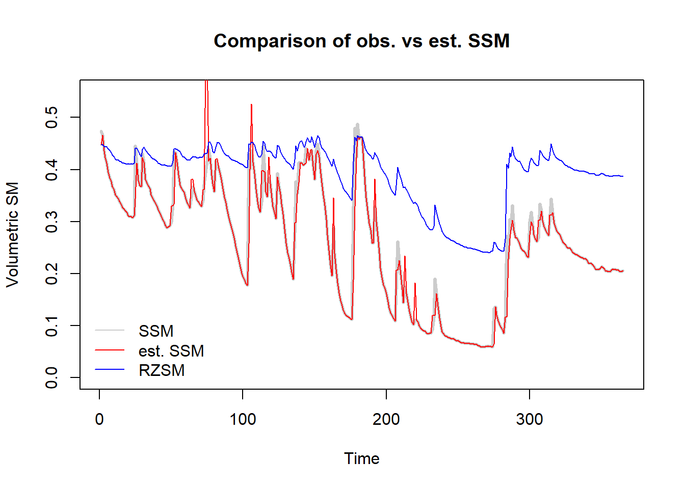
Conversely, the low-pass filter can be inverted to estimate the surface soil moisture using the rootzone soil moisture in an iterative form. Use of this equation can be very helpful in a scenario where surface soil moisture observations are available (for example, from remote-sensing observations) and a simplistic representation of soil water balance for the profile can simultaneously generate equivalent surface soil moisture estimates for model training and validation.
# Inverting low pass filter for SSM estimation from filtered time seriesDp=0.1buffer=0.01*(max(SSM)-min(SSM)) # To decrease sensitivity to noise in sensor readings (1% of SSM range)invLP_filt=function(RZSM){ SSMest=c() SSMest[1]=RZSM[1]for (t in2:length(RZSM)){ SSMest[t]=ifelse(RZSM[t]>(RZSM[t-1]+buffer),min(RZSM[t],SSMf_1[t-1]), (SSMf_1[t-1]+((SSMf_1[t]-SSMf_1[t-1])/Dp))) }return(SSMest)}# Apply LP filter inversionSSMest=invLP_filt(RZSM)# Plot observed v/s estimated Surface soil moisture{plot(SSM, type="l", col="gray80", lwd=3, ylab="Volumetric SM", xlab="Time", main="Comparison of obs. vs est. SSM", ylim=c(0,0.55))lines(SSMest, col="red")lines(RZSM, col="blue")legend(x ="bottomleft", legend =c("SSM", "est. SSM", "RZSM"), lty =c(1,1,1), col =c("gray80","red","blue"), lwd =1, bty ="n") }
Estimating rootzone soil moisture using a low-pass filter and surface soil moisture is efficient but challenging due to the lack of spatially contiguous rootzone soil moisture records for filter calibration. Observations of rootzone soil moisture are only available through a sparse network of observation stations. Some studies use land-surface model simulations for this purpose, but these can only replicate the pre-defined functional relationships in the models and are affected by significant disagreements between models due to different treatments of subgrid-scale heterogeneity in soil and vegetation properties. Additionally, the “active” rootzone layer, which is crucial for root-water uptake and land-atmosphere interactions, varies significantly across different regions. This variability is influenced by factors such as climate (temperature, radiation, and precipitation patterns), vegetation (rooting patterns and water uptake depth), and landscape characteristics (albedo and soil type). In contrast, most land-surface models assume a fixed rootzone depth, typically between 1 and 2 meters.