11  Landscape Soil Hydrology Model

12 Landscape Soil Hydrology Model

12.1 Model Description

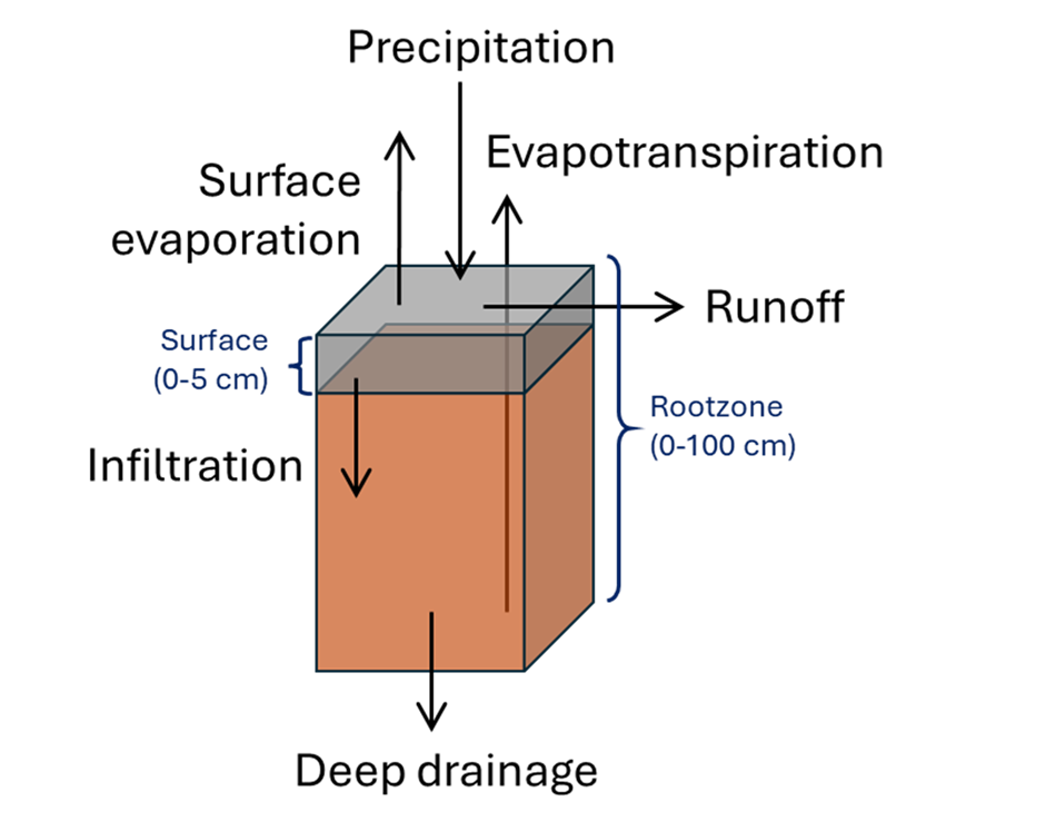
Landscape-scale Soil Hydrology Model is a 2-layer soil water balance model which works based on the emergent signature of terrestrial water-energy coupling beyond the pedon scale scale. As general schematic of the model with key model variables is given below:

12.1.1 Background

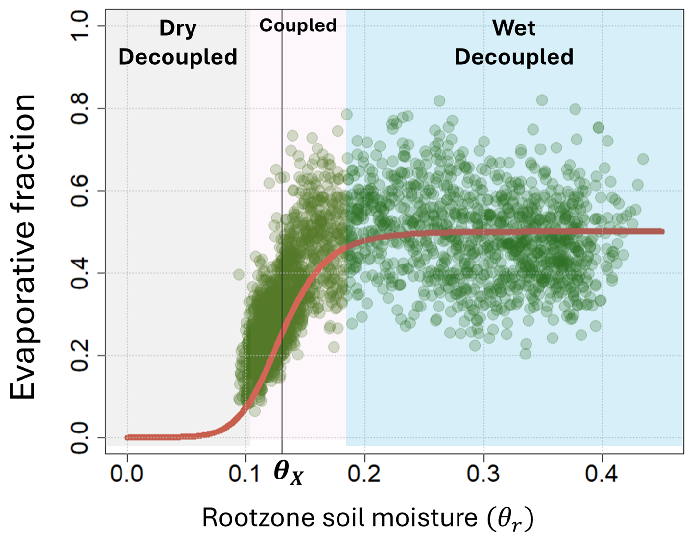
The nature of the soil-vegetation-atmosphere (SVA) interactions evolve with changes in the rootzone soil moisture. This transition of soil hydrologic state from energy-limited to water-limited regimes is represented as a sigmoid curve, with three distinct phases. Abundance of soil moisture in the SVA system can be characterized as wet decoupled, characterized by weakened linkages between water–carbon–energy cycles due to limiting net radiation and atmospheric resistance, with ET losses close to (or at) the potential rate. As the soil begins to dry, soil moisture has higher control over the temporal variability of ET and is characterized by strong land-atmospheric coupling. As soil dries further, soil moisture can not sustain high atmospheric moisture demand, and evapotranspiration again decouples from the rootzone soil moisture.

The connections between soil water balance, noise-induced variability in climatic forces, and positive land-atmospheric feedback lead to dynamic transitions in soil moisture, potentially resulting in a preferred hydrologic states. When one or more state variables are disturbed, or stress (such as atmospheric moisture demand causing evapotranspirative losses) is gradually increased, the SVA system may shift into a new hydrologic regime. Sustained dry-average conditions reinforce dry anomalies (low evaporation results in low regional precipitation and dry soils, leading to even lower evaporation). Conversely, precipitation can alter the soil hydrologic state to wet-average conditions, thereby increasing regional evaporation and precipitation through moisture recycling. If \(\theta_{r}\) represents rootzone soil moisture, then the threshold at which hydrologic tipping of rootzone soil moisture from wet-to-dry-preferential state occurs is represented at \(\theta_{X, r}\), which is called the “tipping” point of the rootzone soil hydrological regimes (Sehgal and Mohanty 2024).

This relationship between rootzone soil moisture and evaporative fraction (evapotranspiration over potential evapotranspiration) is represented as a sigmoid function given below:

\[ EF=\frac{ET}{PET}=\frac{EF_{r,mx}}{\left(1+\left|\left(\frac{\theta_{X, r}\left(\theta_r-1\right)}{\left(1-\theta_{X, r}\right) \theta_r}\right)\right|^m\right)} \]

Here, \(EF_{r,mx}\) represents the maximum evaporative fraction sustainable by the SVA system. The tipping point of soil moisture is represented as \(\theta_{X}\). Land-atmospheric coupling strength is represented by the parameter \(m\). The input vertical flux to the soil below the surface is considered to be derived from the drainage of the surface profile, which is a non-linear function of the field capacity \(\theta_{fc}\), saturated hydraulic conductivity (\(K_{s}\)), porosity (\(\eta\)) and an empirical power coefficient, \(b\). The same equation is adopted for the rootzone to estimate deep drainage.

\[ D=K_S\left(\frac{\left(\max \left(0, \theta-\theta_{f c}\right)\right)}{\eta-\theta_{f c}}\right)^b \]

Surface runoff is estimated as the saturation excess component of the precipitation, based on the hydrologic state of the surface profile. Surface evaporation is considered as a fraction \(Es_{frac}\) of the net evapotranspiration. The depth of the surface and the rootzone profile are fixed and are assumed to be 0-5 and 0-100 cm respectively.

12.1.2 Priestley-Taylor Method for Potential ET (PET)

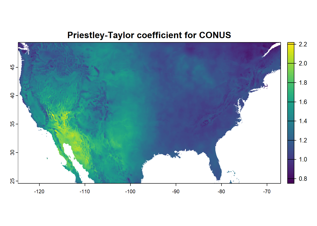
The model uses Priestley-Taylor equation for potential ET estimation. This formulation is based on physical principles and can be seen as a simplified version of the Penman-Monteith formula for calculating evapotranspiration. The simplification involves removing the aerodynamic terms from the Penman-Monteith equation and using a constant (\(α\)), which has been empirically derived and is estimated to be 1.26 for open bodies of water, but can range from <1 (humid conditions) to almost 2 (arid conditions). This constant tends to be higher in arid regions or areas experiencing significant water stress. The Priestley-Taylor formula can be used for calculating daily evapotranspiration and can also be applied to smaller time intervals (hourly, for example) if the necessary data is available.

\[ \text { PET }=\left(\frac{\alpha}{\lambda_v \rho_{\mathrm{w}}}\right) \times \frac{\Delta}{\Delta+\gamma} \times \text {R} \]

if \(T_{mean}< 0^oC\)

\[ \Delta=0.3405 \times \mathrm{e}^\left(0.0642 \mathrm{~T}_{\text {mean}}\right) \\ \]

if \(T_{mean}> 0^oC\) \[ \Delta=0.3221 \times \mathrm{e}^\left(0.0803 \mathrm{~T}_{\mathrm{mean}}^{0.8876}\right) \]

where,

\(PET\)= Daily potential evapotranspiration (\(m\))

\(λv\) = Latent heat of vaporization (2260 \(kJ/kg\))

\(ρw\) = Density of water (1000 \(kg/m^3\))

\(γ\) = Psychrometric constant ( 4.95x \(10^{-4}\) \(kg/m^3/^oC\))

\(Rad\) = Daily solar radiation incident on a horizontal earth surface (\(kg/m^2\))

\(Δ\) = Slope of the saturation vapor density curve from the psychrometric chart (\(kg/^oC\))

\(T_{mean}\) = Daily mean air temperature (\(^oC\))

\(\alpha\) = Priestley-Taylor correction factor

For use with this model, we will use global, high resolution (30arc-sec) estimates of PT correction factor from (Aschonitis et al. 2017). The dataset will be masked to the extent of the region-of-interest at the time of model implementation. Let’s view the values of Priestley-Taylor correction factor for Contiguous US.

library(terra)
utils::download.file("https://github.com/Vinit-Sehgal/SampleData/blob/master/raster_files/priestley_taylor_coefficient/cropPTalpha.tif?raw=true",
                     destfile = "cropPTalpha.tif", 
                     mode="wb", #wb is write binary
                     method ='auto', 
                     quiet=FALSE)
PTalpha=rast("cropPTalpha.tif")
plot(PTalpha, main="Priestley-Taylor coefficient for CONUS")

12.2 Catchment Hydrology with LaSH model

12.2.1 MOPEX Catchments

MOPEX (Model Parameter Estimation Experiment, (Schaake, Cong, and Duan 2006)) catchments are a collection of hydrological catchments across the continental United States used for studying and modeling various aspects of hydrology. These catchments are part of a large dataset that includes daily measurements of evaporation, precipitation, streamflow, and temperature, along with other properties such as drainage area, elevation, and slope. The primary goal of the MOPEX initiative is to improve the understanding and prediction of hydrological processes by providing a comprehensive dataset for model calibration and validation. We will use one of the MOPEX catchments in Louisiana for the demonstration of LaSH model at catchment scale (Duan et al. 2006).

library(terra)   # for spatial data manipulation
library(mapview) # for spatial data visualization

MOPEX=vect("./SampleData-master/MOPEX/MOPEX_catchments_431.shp")

# Display the MOPEX catchments
mapview(MOPEX, col.regions="blue", lwd=2, legend=TRUE, layer.name="MOPEX Catchments")  
# List of LA catchments: 107, 427, 141, 406, 185
mymopex=MOPEX[427,1]
plot(mymopex, col="gray88", lwd=2, main="Selected catchment in Louisiana")

# Extract the extent of the catchment. We will download Met data matching this extent
mopex_ext=ext(mymopex) 

12.2.2 Meteorological Variables

One might recollect Daymet dataset from Chapter 6. We will use Daymet dataset, version 4 (Thornton et al. 1850) as a source of high-resolution, daily surface weather data for the sample catchment. This dataset offers gridded estimates of various weather parameters such as: Minimum and maximum temperature, Precipitation, Shortwave radiation, Vapor pressure, Snow water equivalent and Day length. Appropriate transformation is applied to the dataset to transform the variables to the necessary units.

The data is available at a 1 km x 1 km spatial resolution and covers the period from January 1, 1980, to the most recent full calendar year. As an example, we will use daily gridded dataset for the year 2018 for precipitation (prcp, in mm), maximum/minimum daily temperature (tmax/tmin, in degree C),Shortwave radiation (srad, in W m-2).

############################################################################################
# Meteorological dataset
############################################################################################
# Download 1-km meteorological data for the selected catchment 
library("daymetr") 

# prcp (mm)
download_daymet_ncss(location = c(mopex_ext[4],mopex_ext[1],mopex_ext[3],mopex_ext[2]),
                     # location = bounding box extent defined as top left / bottom right pair c(lat,lon,lat,lon)
                     start = 2018,
                     end = 2018,
                     path = tempdir(),  # Save file in the temp directory
                     param = "prcp", 
                     silent = TRUE)
# srad (W m-2)
download_daymet_ncss(location = c(mopex_ext[4],mopex_ext[1],mopex_ext[3],mopex_ext[2]),
                     # location = bounding box extent defined as top left / bottom right pair c(lat,lon,lat,lon)
                     start = 2018,
                     end = 2018,
                     path = tempdir(),  # Save file in the temp directory
                     param = "tmax", 
                     silent = TRUE)
# tmin (degree C)
download_daymet_ncss(location = c(mopex_ext[4],mopex_ext[1],mopex_ext[3],mopex_ext[2]),
                     # location = bounding box extent defined as top left / bottom right pair c(lat,lon,lat,lon)
                     start = 2018,
                     end = 2018,
                     path = tempdir(),  # Save file in the temp directory
                     param = "tmin", 
                     silent = TRUE)
# tmax (degrees c)
download_daymet_ncss(location = c(mopex_ext[4],mopex_ext[1],mopex_ext[3],mopex_ext[2]),
                     # location = bounding box extent defined as top left / bottom right pair c(lat,lon,lat,lon)
                     start = 2018,
                     end = 2018,
                     path = tempdir(), # Save file in the temp directory
                     param = "srad", 
                     silent = TRUE)


prcpYr=0.1*rast(file.path(tempdir(),"prcp_daily_2018_ncss.nc"))     # in cm/day
tmaxYr=rast(file.path(tempdir(),"tmax_daily_2018_ncss.nc"))         # in deg C
tminYr=rast(file.path(tempdir(),"tmin_daily_2018_ncss.nc"))         # in deg C
sradYr=86.400*rast(file.path(tempdir(),"srad_daily_2018_ncss.nc"))  # in KJ/m2/day

############################################################################################
# Reproject to the projection of the catchment
pcpProj=terra::project(prcpYr, crs(mymopex))
tmaxProj=terra::project(tmaxYr, crs(mymopex))
tminProj=terra::project(tminYr, crs(mymopex))
sradProj=terra::project(sradYr, crs(mymopex))

############################################################################################
# Crop to the catchment extent
############################################################################################
pcpcrp=crop(pcpProj,mymopex, mask=T)
tmaxcrp=crop(tmaxProj,mymopex, mask=T)
tmincrp=crop(tminProj,mymopex, mask=T)
sradcrp=crop(sradProj,mymopex, mask=T)

############################################################################################
# Priestley-Taylor correction factor
############################################################################################
PTalpha=rast("C:/Users/VSehgal/OneDrive - LSU AgCenter/TAMU/research_tamu/general_data_access/priestley_taylor_coefficient/cropPTalpha.tif")
PTalphaProj=terra::project(PTalpha, crs(mymopex))
ptalphacrp=crop(PTalphaProj,mymopex, mask=T)
alpha=resample(ptalphacrp,pcpcrp)
names(alpha)="PTcoefficient"

plot(alpha, main="PT correction factor for the catchment")
plot(mymopex, add=T)

12.3 Random Fields of Soil and Land-Atmosphere Coupling Parameters

We will use random values of input model variables for the implementation of the model for the catchment. We will add a synthetic diagonal gradient in the model parameters to represent spatial heterogeneity in the model parameters within the catchment. The list of model parameters and their description is given in the table below.

Abbreviation Description
SMrx Rootzone crossing point
mr LA coupling strength
EFrmx Max rootzone Evaporative fraction
Es_frac Surface evaporation fraction: E/Total ET
por_s Surface porosity
por_r Rootzone porosity
b_s Power coefficient of surface drainage curve
b_r Power coefficient of rootzone drainage curve
Ks_s Surface Saturated hydraulic conductivity
Ks_r Rootzone Saturated hydraulic conductivity
fc_s Surface field capacity
############################################################################################
# Create synthetic fields of soil hydraulic and land-atmospheric coupling params
############################################################################################
# Create a field with diagonal gradient 
x = seq(0,1,len=10)
y = seq(0,1,len=10)

randmRast = rast(outer(x,y,function(x,y){(0.1*(x)+0.1*(y))}))
# Create anomaly w.r.t mean values of the sample raster
randmano=(randmRast-as.numeric(global(randmRast, mean, na.rm = T)))
plot(randmano)  

# Mask and re-project the synthetic raster to the catchment
ext(randmano)=ext(mymopex)
crs(randmano)=crs(mymopex)
# Resample the synthetic raster to the resolution of the meteorological data
anomaly_resamp=resample(randmano,pcpcrp)
anomaly_crp=crop(anomaly_resamp, mymopex, mask=T)

# Mean value of model parameters for the catchment
SMrx=0.30      # Rootzone crossing point 
mr=2.5         # LA coupling strength    
EFrmx=0.8      # Max rootzone Evaporative fraction 
Es_frac=0.15   # Surface evaporation fraction: E/Total ET
por_s=0.44     # Surface porosity
por_r=0.52     # Rootzone porosity  
b_s=12         # Power coefficient of surface drainage curve
b_r=0.8        # Power coefficient of rootzone drainage curve 
Ks_s=0.14      # Surface Saturated hydraulic conductivity 
Ks_r=0.9       # Rootzone Saturated hydraulic conductivity 
fc_s=0.4       # Surface field capacity

par_mean= c(SMrx, mr, EFrmx, Es_frac, por_s, por_r, b_s, b_r, Ks_s, Ks_r, fc_s)

# Generate rasters to store spatially distributed values for each parameter
parRas=rep(rast(anomaly_crp),11)            # Create empty raster stack
values(parRas)=rep(values(anomaly_crp),11)  # Fill the raster stack with the anomaly values
names(parRas)= c("SMrx","mr","EFrmx","Es_frac",
                 "por_s","por_r","b_s","b_r","Ks_s", "Ks_r","fc_s")

# Impose anomalies on the mean values of the model parameters
parDist=parRas*par_mean+par_mean 
plot(parDist, fun=function(){plot(mymopex, add=T)})

12.4 Model Application for the catchment

Using the dataset and model parameters, we will apply the LaSH model to each grid to generate spatially distributed outputs of hydrological variables.

############################################################################################
# Soil Water Balance Model
############################################################################################
# Soil moisture values for model initiation
ini_cond=rast(pcpcrp[[1]]) # Generate empty raster to store values using PCP raster as sample
values(ini_cond)=0.25      # Initial soil moisture condition
names(ini_cond)="ini_condition"

# Create a raster stack with all input parameters
ParInRas=c(parDist, ini_cond, alpha) 
# Create a raster stack with all forcing variables
forcingRas=c(pcpcrp, (tmaxcrp+tmincrp)/2, sradcrp) 
SWB_model=function(ParIn,forcing){
  
  # Input parameters  
  SMrx=ParIn[1]         # Rootzone crossing point 
  mr=ParIn[2]           # LA coupling strength  
  EFrmx=ParIn[3]        # Max rootzone Evaporative fraction 
  Es_frac=ParIn[4]      # Surface evaporation fraction: E/Total ET
  
  por_s=ParIn[5]        # Surface porosity
  por_r=ParIn[6]        # Rootzone porosity
  b_s=ParIn[7]          # Power coefficient of surface drainage curve
  b_r=ParIn[8]          # Power coefficient of rootzone drainage curve
  Ks_s=ParIn[9]         # Surface Saturated hydraulic conductivity 
  Ks_r=ParIn[10]        # Rootzone Saturated hydraulic conductivity 
  fc_s=ParIn[11]        # Surface field capacity
  
  ini_condition=ParIn[12]        # Initial SM condition 
  alphaVal= ParIn[13]            # Priestley-Taylor coefficient
  
  spinup=20             # Excluded from the model evaluation
  zs=5                  # Surface layer depth (cm)
  zr=95                 # Difference between rootzone and surface profile depth (cm)
  
  # Rootzone SWRP
  fc_r=SMrx+EFrmx/(2*mr)
  wp_r=pmax(0.02,(SMrx-EFrmx/(2*mr)))
  
  # Forcings
  PCP=forcing[1:(length(forcing)/3)]
  Tmean=forcing[(1+(length(forcing)/3)): (2*(length(forcing)/3))]
  Rad=forcing[(2*(length(forcing)/3)+1):length(forcing)]
  
  PT_PET<<-function(Tmean,Rad,alpha){
    lambdaV= 2260                  # Latent heat of vaporization 
    rhoW= 1000                     # Density of water 
    gamma= 4.95*1e-4               # Psychrometric constant
    
    deltaVal=rep(0, length(Tmean))  # Create empty array
    
    # When Tmean<0
    deltaVal[Tmean<0]=0.3405*exp(0.0642*Tmean[Tmean<0])
    # When Tmean>=0
    deltaVal[Tmean>=0]=0.3221*exp(0.0803*((Tmean[Tmean>=0])^0.8876))
    
    # Priestley-Taylor equation 
    PETval=(alpha/(lambdaV*rhoW))*(deltaVal/(deltaVal+gamma))*Rad
    PETval[PETval<0]=0
    return(PETval) #estimate in m
  }
  
  #~~~ Simple Soil Water Balance Model 
  # Empty arrays to store data
  RZSM= SSM= drainage= ETr= ETs=PET= runoff= infilt =infilCap=c()  
  SSM[1]= RZSM[1]= ini_condition            # Initial soil moisture state
  for (t in 2:length(PCP)){
    
    infilCap[t]= pmax(0,(por_s-SSM[t-1])*zs)
    runoff[t]=pmax(0,(PCP[t]-infilCap[t]))
    
    infilt[t]= Ks_s*(pmax(0,SSM[t-1]-fc_s)/(por_s-fc_s))^b_s
    SSM[t]=pmin(por_s,(pmax(0.02,
                            (zs*SSM[t-1]+pmin(PCP[t],infilCap[t])-infilt[t])/zs)))
    
    # 4. Calculate surface evaporation for days with no PCP 
    PET[t]=100*PT_PET(Tmean[t],Rad[t],alpha=alphaVal)  #PET in cm
    
    # Estimate ET based on PET and RZSM state
    ETr[t]=PET[t]*EFrmx/(1+(abs((SMrx*(RZSM[t-1]-1))/(RZSM[t-1]*(1-SMrx))))^mr)
    ETs[t]=Es_frac*ETr[t]
    
    # 5. Exclude evaporative losses from SSM
    SSM[t]=ifelse(PCP[t]==0,
                  pmin(por_s,pmax(0.02,(zs*SSM[t]-ETs[t])/zs)),SSM[t])
    
    # Deep drainage based on RZSM state. Continues till CP
    drainage[t]= Ks_r*(pmax(0,RZSM[t-1]-fc_r)/(por_r-fc_r))^b_r
    
    # Update RZSM after drainage and ET
    RZSM[t]=pmin(por_r,pmax(wp_r,
                            ((zr+zs)*RZSM[t-1]+zs*SSM[t]-drainage[t]-ETr[t]+infilt[t])/(zr+zs))) 
  }
  # Return the model output
  return(c(SSM,RZSM,infilt, drainage,ETr,ETs, runoff,PET))
}

############################################################################################
# Model implementation for sample location
############################################################################################
sampLoc=cbind(-91.15,30.8)                           # Sample location for model evaluation
parTS=as.numeric(extract(ParInRas, sampLoc))         # Extract model parameters for the location
forcingTS=as.numeric(extract(forcingRas, sampLoc))   # Extract forcing variables for the location

# Model output for the sample location
outTS=SWB_model(parTS,forcingTS) 

# Extract time series of simulated variables
{ i=0; SSMTS=outTS[(365*i+1):(365*(i+1))]
  i=1; RZSMTS=outTS[(365*i+1):(365*(i+1))]
  i=2; infiltTS=outTS[(365*i+1):(365*(i+1))]
  i=3; drainageTS=outTS[(365*i+1):(365*(i+1))]
  i=4; ETrTS=outTS[(365*i+1):(365*(i+1))]
  i=5; ETsTS=outTS[(365*i+1):(365*(i+1))]
  i=6; runoffTS=outTS[(365*i+1):(365*(i+1))]
  i=7; PETTS=outTS[(365*i+1):(365*(i+1))]} 

# Plot surface soil moisture
plot(SSMTS, type="l", ylim=c(0,0.55), 
     ylab="Simulated soil moisture", 
     xlab="Time (days)")             
# add rootzone soil moisture
lines(RZSMTS, type="l",col="red")                 
legend(x = "topleft", legend=c("SSM", "RZSM"), 
      bg ="transparent",box.col = "transparent",
      fill = c("black","red")) 

############################################################################################
# Model implementation for the catchment
############################################################################################
modelOut = terra::xapp(ParInRas, forcingRas, fun= SWB_model)     # Model output for the catchment

# Gather simulated variables
{i=0; SSM=modelOut[[(365*i+1):(365*(i+1))]]; names(SSM)=paste("day",seq(1:365))
i=1; RZSM=modelOut[[(365*i+1):(365*(i+1))]]; names(RZSM)=paste("day",seq(1:365))
i=2; infilt=modelOut[[(365*i+1):(365*(i+1))]]; names(infilt)=paste("day",seq(1:365))
i=3; drainage=modelOut[[(365*i+1):(365*(i+1))]]; names(drainage)=paste("day",seq(1:365))
i=4; ETr=modelOut[[(365*i+1):(365*(i+1))]]; names(ETr)=paste("day",seq(1:365))
i=5; ETs=modelOut[[(365*i+1):(365*(i+1))]]; names(ETs)=paste("day",seq(1:365))
i=6; runoff=modelOut[[(365*i+1):(365*(i+1))]]; names(runoff)=paste("day",seq(1:365))
i=7; PET=modelOut[[(365*i+1):(365*(i+1))]]; names(PET)=paste("day",seq(1:365))} 

# Plot the model output for a sample day
{n=108                 # Day of interest
dayOut=c(SSM[[n]],
         RZSM[[n]],
         infilt[[n]],
         drainage[[n]],
         ETr[[n]],
         ETs[[n]],
         runoff[[n]],
         PET[[n]])
names(dayOut)=c("SSM","RZSM","infilt","drainage","ETr","ETs","runoff","PET")
plot(dayOut)} 

# Plot simulated RZSM for the first 10 days
plot(RZSM[[1:10]], range=c(0.25,0.40), fun=function(){plot(mymopex, add=T)}) 

#Extract time series of simulated variables for the sample location
{ SSMts=as.numeric(extract(SSM, sampLoc))
  RZSMts=as.numeric(extract(RZSM, sampLoc))
  infiltts=as.numeric(extract(infilt, sampLoc))
  drainagets=as.numeric(extract(drainage, sampLoc))
  ETrts=as.numeric(extract(ETr, sampLoc))
  ETsts=as.numeric(extract(ETs, sampLoc))
  runoffts=as.numeric(extract(runoff, sampLoc))
  PETts=as.numeric(extract(PET, sampLoc))}

plot(ETrts, type="l", main="Simulated ET for the location",
     xlab="Time (days)", ylab="ET (cm/day)")

12.5 Field Application of LaSH Model

We will use sample dataset from a CRN site to demonstrate the application of LaSH model for field-scale applications.

############################################################################################
# Data Access for Sample Location
############################################################################################
library(zoo)
utils::download.file("https://github.com/Vinit-Sehgal/SampleData/blob/master/CRN_data/CRND0103-2021-OK_Stillwater_2_W.txt?raw=true",
                     destfile = "CRND0103-2021-OK_Stillwater_2_W.txt", 
                     mode="wb", #wb is write binary
                     method ='auto', 
                     quiet=FALSE) #


utils::download.file("https://github.com/Vinit-Sehgal/SampleData/blob/master/CRN_data/HEADERS.txt?raw=true",
                     destfile = "headers.txt", 
                     mode="wb", #wb is write binary
                     method ='auto', 
                     quiet=FALSE)
CRNdat = read.csv("CRND0103-2021-OK_Stillwater_2_W.txt", header=FALSE,sep="")
headers = read.csv("headers.txt", header=FALSE,sep="")

# Column names as headers from the text file
colnames(CRNdat)=headers[2,1:ncol(CRNdat)]

# Replace fill values with NA
CRNdat[CRNdat == -9999]=NA
CRNdat[CRNdat == -99]=NA
CRNdat[CRNdat == 999]=NA

# Weighted average of soil moisture at multiple depths to estimate RZSM
SMpdf=data.frame(
  SM5=na.approx(CRNdat$SOIL_MOISTURE_5_DAILY,na.rm = FALSE), 
  SM10=na.approx(CRNdat$SOIL_MOISTURE_10_DAILY,na.rm = FALSE), 
  SM20=na.approx(CRNdat$SOIL_MOISTURE_20_DAILY,na.rm = FALSE), 
  SM50=na.approx(CRNdat$SOIL_MOISTURE_50_DAILY,na.rm = FALSE),
  SM100=na.approx(CRNdat$SOIL_MOISTURE_100_DAILY,na.rm = FALSE))

SSM_obs=SMpdf$SM5; 
RZSM_obs=(SMpdf$SM5*(7.5-0)+            # 0- 7.5 cm depth
            SMpdf$SM10*(15-7.5)+        # 7.5-15 cm depth
            SMpdf$SM20*(35-15)+         # 15-35 cm depth
            SMpdf$SM50*(75-35)+         # 35-75 cm depth
            SMpdf$SM100*(100-75))/100   # 75-100 cm depth

# Target location
coord=cbind(CRNdat$LONGITUDE[1], CRNdat$LATITUDE[1]) 

############################################################################################
# Setting Model Parameters and Forcing Data
############################################################################################
# Set condition for model initiation
ini_condition=RZSM_obs[which(!is.na(RZSM_obs))[1]]
spinup=10            # Excluded from the model evaluation
zs=5                 # Surface layer depth (cm)
zr=95                # Rootzone profile depth (cm)

# Trial parameters for model run
SMrx=0.127        # Rootzone crossing point 
mr=10             # LA coupling strength 
EFrmx=0.59        # Max rootzone Evaporative fraction 
Es_frac=0.108     # Surface evaporation fraction: E/Total ET
por_s=0.429       # Surface porosity
por_r=0.458       # Rootzone porosity
b_s=7.768         # Power coefficient of surface drainage curve
b_r=6.040         # Power coefficient of rootzone drainage curve
Ks_s=0.280        # Surface Saturated hydraulic conductivity 
Ks_r=2.601        # Rootzone Saturated hydraulic conductivity 
fc_s=0.405        # Surface field capacity

parIn=c(SMrx,mr,EFrmx,Es_frac,por_s,por_r,b_s,b_r,Ks_s,Ks_r,fc_s)

# Priestley-Taylor correction factor for the location
alphaVal=as.numeric(terra::extract(PTalpha,coord),method='bilinear'); alphaVal
[1] 1.37
# Data frame with Met forcings
forcing=data.frame(Rad=CRNdat$SOLARAD_DAILY*1000,    # in KJ
                   Tmean=CRNdat$T_DAILY_MEAN,        # in deg C  
                   PCP=CRNdat$P_DAILY_CALC/10)       # in cm
head(forcing)
    Rad Tmean  PCP
1  3510   1.2 2.30
2  7020   2.2 0.00
3 10560   2.7 0.00
4 11130   5.7 0.00
5  9990   6.3 0.00
6  1030   7.2 0.03

We will modify the SWB model function shown earlier for application to single station application. Instead of stacking all output variables, this form collate the columns and give a 2-D matrix of the simulated variables, with each column representing one variable.

############################################################################################
# Soil Water Balance Model Function
############################################################################################
SWB_model=function(ParIn,ini_condition,forcing){
  
  # Input parameters  
  SMrx=ParIn[1]         # Rootzone crossing point 
  mr=ParIn[2]           # LA coupling strength  
  EFrmx=ParIn[3]        # Max rootzone Evaporative fraction 
  Es_frac=ParIn[4]      # Surface evaporation fraction: E/Total ET
  
  por_s=ParIn[5]        # Surface porosity
  por_r=ParIn[6]        # Rootzone porosity
  b_s=ParIn[7]          # Power coefficient of surface drainage curve
  b_r=ParIn[8]          # Power coefficient of rootzone drainage curve
  Ks_s=ParIn[9]         # Surface Saturated hydraulic conductivity 
  Ks_r=ParIn[10]        # Rootzone Saturated hydraulic conductivity 
  fc_s=ParIn[11]        # Surface field capacity
  
  # Rootzone SWRP
  fc_r=SMrx+EFrmx/(2*mr)
  wp_r=pmax(0.02,(SMrx-EFrmx/(2*mr)))
  
  # Forcings
  PCP=na.approx(forcing$PCP, na.rm=F)
  Tmean=na.approx(forcing$Tmean, na.rm=F)
  Rad=na.approx(forcing$Rad, na.rm=F)
  
  # PET estimation using Priestley-Taylor method 
    PT_PET=function(Tmean,Rad,alpha){
      lambdaV= 2260                  # Latent heat of vaporization 
      rhoW= 1000                     # Density of water 
      gamma= 4.95*1e-4               # Psychrometric constant
      
      deltaVal=rep(0, length(Tmean))  # Create empty array
      
      # When Tmean<0
      deltaVal[Tmean<0]=0.3405*exp(0.0642*Tmean[Tmean<0])
      # When Tmean>=0
      deltaVal[Tmean>=0]=0.3221*exp(0.0803*((Tmean[Tmean>=0])^0.8876))
      
      # Priestley-Taylor equation 
      PETval=(alpha/(lambdaV*rhoW))*(deltaVal/(deltaVal+gamma))*Rad
      PETval[PETval<0]=0
      return(PETval) #estimate in m
    }

  #~~~ Simple Soil Water Balance Model 
  # Empty arrays to store data
  RZSM= SSM= drainage= ETr= ETs=PET= runoff= infilt =infilCap=c()  
  SSM[1]= RZSM[1]= ini_condition            # Initial soil moisture state
  for (t in 2:length(PCP)){
    
    infilCap[t]= pmax(0,(por_s-SSM[t-1])*zs)
    runoff[t]=pmax(0,(PCP[t]-infilCap[t]))
    
    infilt[t]= Ks_s*(pmax(0,SSM[t-1]-fc_r)/(por_s-fc_r))^b_s
    SSM[t]=pmin(por_s,(pmax(0.02,
                            (zs*SSM[t-1]+pmin(PCP[t],infilCap[t])-infilt[t])/zs)))
    
    # 4. Calculate surface evaporation for days with no PCP 
    PET[t]=100*PT_PET(Tmean[t],Rad[t],alpha=alphaVal)  #PET in cm
    
    # Estimate ET based on PET and RZSM state
    ETr[t]=PET[t]*EFrmx/(1+(abs((SMrx*(RZSM[t-1]-1))/(RZSM[t-1]*(1-SMrx))))^mr)
    ETs[t]=Es_frac*ETr[t]
    
    # 5. Exclude evaporative losses from SSM
    SSM[t]=ifelse(PCP[t]==0,
                  pmin(por_s,pmax(0.02,(zs*SSM[t]-ETs[t])/zs)),SSM[t])
    
    # Deep drainage based on RZSM state. Continues till CP
    drainage[t]= Ks_r*(pmax(0,RZSM[t-1]-fc_r)/(por_r-fc_r))^b_r
    
    # Update RZSM after drainage and ET
    RZSM[t]=pmin(por_r,pmax(wp_r,
                            ((zr+zs)*RZSM[t-1]+zs*SSM[t]-drainage[t]-ETr[t]+infilt[t])/(zr+zs))) 
  }
  return(cbind(SSM,RZSM,infilt, drainage,ETr,ETs, runoff,PET))
}

# Apply the SWB model on test dataset
  optimOut=SWB_model(ParIn=parIn, 
                     ini_condition=RZSM_obs[which(!is.na(RZSM_obs))[1]],
                     forcing=forcing)
  
  # Convert the output array to a data frame for easy plotting
  optimOut=data.frame(optimOut) 
  
  # Add time and precipitation to the output df so it can be plotted 
  optimOut$PCP=forcing$PCP
  optimOut$time=as.Date(as.character(CRNdat$LST_DATE),format="%Y%m%d")
  optimOut$RZSM_obs=RZSM_obs
  optimOut$SSM_obs=SMpdf$SM5

Now that we have executed the model for the sample dataset, we will plot the simulated variables. We will also overlay the observed surface and rootzone soil moisture to compare the ability of the model in simulaing temporal dynamics of the observed variables. ::: {.cell}

############################################################################################
# Plot Simulated Variables
############################################################################################
  library(ggplot2)
  library(patchwork)
  
  # Plot for observed and modeled RZSM
  p_SSM=ggplot(optimOut) +
    geom_line(aes(x = time, y = SSM, color = "SSM"),linetype=2)+
    geom_line(aes(x = time, y = SSM_obs, color = "SSM_obs"),linetype=1)+
    scale_y_continuous( name = "SSM")+
    labs(x = "Time") +
    theme_minimal() +
    scale_color_manual(values = c("blue","black"))+
    theme(legend.title = element_blank())
  
  p_RZSM=ggplot(optimOut) +
    geom_line(aes(x = time, y = RZSM, color = "RZSM"),linetype=2)+
    geom_line(aes(x = time, y = RZSM_obs, color = "RZSM_obs"),linetype=1)+
    scale_y_continuous( name = "RZSM")+
    labs(x = "Time") +
    theme_minimal() +
    scale_color_manual(values = c("blue","black"))+
    theme(legend.title = element_blank())
  
  # Plot for modeled ET
  p_ET=ggplot(optimOut) +
    geom_line(aes(x = time, y = ETr, color = "ET"))+
    scale_y_continuous( name = "ET")+
    labs(x = "Time") +
    theme_minimal() +
    scale_color_manual(values = c("ET" = "blue"))+
    theme(legend.title = element_blank())
  
  # Plot for modeled drainage
  p_drain=ggplot(optimOut) +
    geom_line(aes(x = time, y = drainage, color = "drainage"))+
    scale_y_continuous( name = "GW recharge")+
    labs(x = "Time") +
    theme_minimal() +
    scale_color_manual(values = c("drainage" = "blue"))+
    theme(legend.title = element_blank())
  
  # Plot for observed precipitation
  p_PCP=ggplot(optimOut) +
    geom_bar(aes(x = time, y = PCP, fill = "PCP"),  
             stat = "identity")+
    scale_y_continuous( name = "PCP")+
    labs(x = "Time") +
    theme_minimal() +
    scale_fill_manual(values = c("PCP" = "black"))+
    theme(legend.title = element_blank())
  
  # Plot for modeled drainage
  p_runoff=ggplot(optimOut) +
    geom_bar(aes(x = time, y = runoff, fill = "runoff"),stat = "identity")+
    scale_y_continuous( name = "Runoff")+
    labs(x = "Time") +
    theme_minimal() +
    scale_fill_manual(values = c("runoff" = "black"))+
    theme(legend.title = element_blank())

# Combine all plots into a single window
library(patchwork)
p_SSM/p_RZSM/p_PCP/p_runoff/p_ET/p_drain+                # Plots one under the other
  plot_layout(guides = "collect",       # Collect common legends
              axis_titles = "collect",    # Collect common axis titles
              axes="collect") &           # Collect common axis labels
  theme(legend.position='bottom')

:::