5 Spatial Operations on Rasters and Vectors

5.1 Meet the Data

For this chapter, we will use Aridity index (AI), which is a popular metric for climate classification based on the relative availability of Mean Annual Precipitation (P) compared to the Mean Annual Reference Evapotranspiration (ET₀) of a location. Aridity Index is defined as: \(AI= P / ET_0\). Here, ET₀ is the maximum potential amount of moisture a hydrologic system can transfer to atmosphere through evaporation and transpiration. The value of \(P / ET_0\) progressively increases from arid to humid regions. Since P and ET₀ can never be negative, AI is always >0.

Global Climate Classification Map Based on Aridity Index

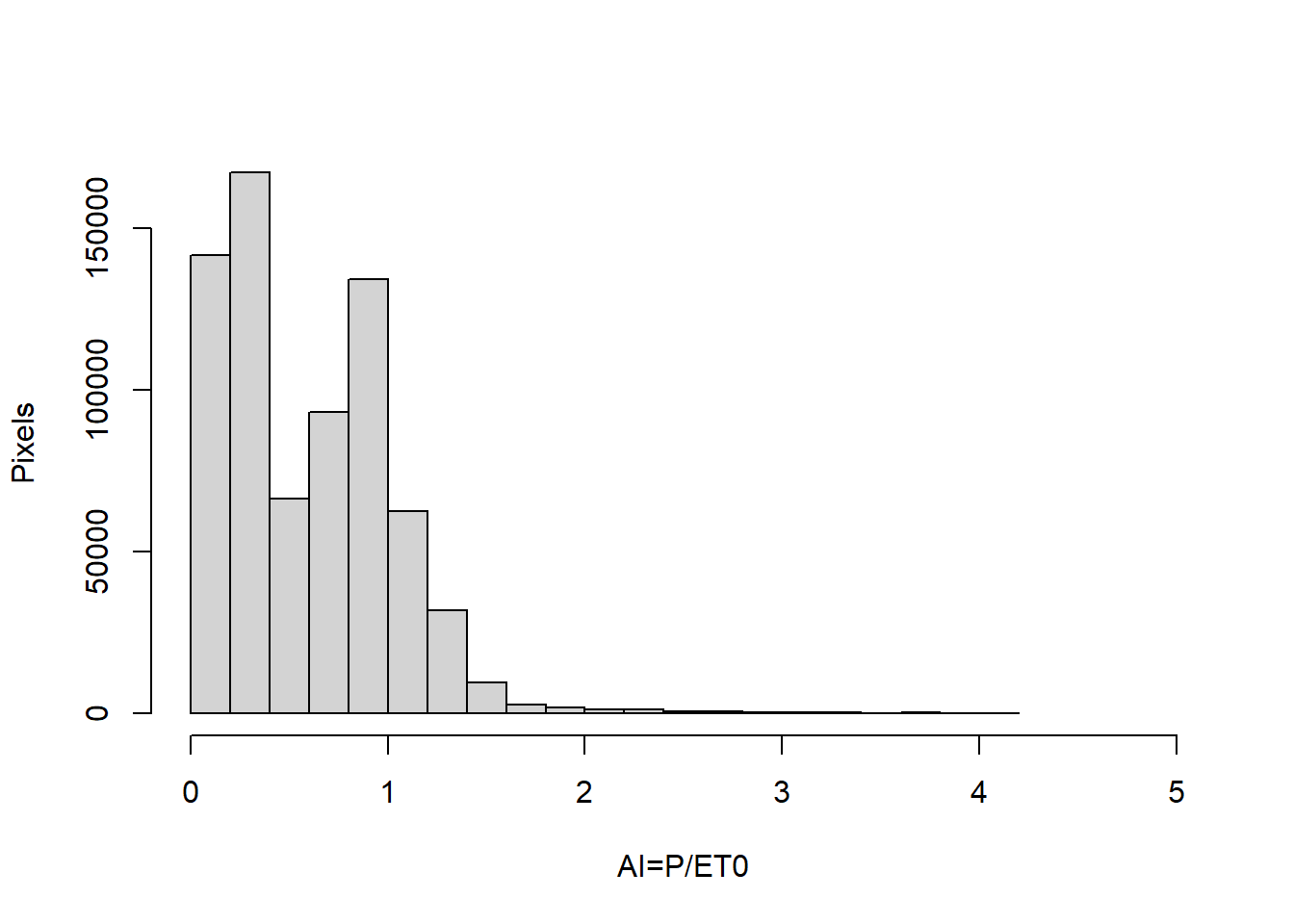
For the purpose of this demonstration, we will use CONUS-wide raster of aridity index estimates (i.e. P/ET₀) provided by (Zomer, Xu, and Trabucco 2022), at ~0.8X0.8 KM spatial resolution. Let us first start by downloading the sample data files (refer to previous chapters for the code). We will then import the raster and plot a histogram of the raster to understand the probability distribution of the AI values. Do we agree that most pixels in the raster range within 0-4?

library(terra)
AI=terra::rast("./SampleData-master/raster_files/P_over_ET0.tif") 

# Let us plot a histogram of the raster
hist(AI, breaks=20, 
     xlim=c(0,5), 
     xlab="AI=P/ET0", 
     ylab="Pixels", main="") 

# We observe most values in the raster are <4. So, we set the range of the plot accordingly
terra::plot(AI, main="AI=P/ET0", range=c(0,4))

5.2 Raster Resampling

We have so far worked with global surface soil moisture raster (from SMAP) and we are familiar with its spatial distribution across the globe. Now, let us consider this question:

How does the climate impact the spatial distribution of soil moisture?

One approach of answering the question can be to compare pixel values of SMAP soil moisture with corresponding values of AI to establish the bivariate AI–SM relationship. So, we must first change the resolution of AI raster to match that of the SMAP soil moisture. For this, we will use raster resampling.

Raster resampling simply refers to making changes to the pixel resolution of the raster. The term “resampling” implies that the pixel values are “sampled” and reassigned to the pixels at the new resolution. This operations often involves an interpolation method (nearest neighbor, bilinear, spline, min, max, mode, average etc). We will try three important functions for changing the resolution of a SpatRaster:

1. terra::resample - resample to match the resolution of another raster

2. terra::aggregate - resample from fine to coarse resolution

3. terra::disagg - resample from coarse to fine resolution

Raster resampling can be a critical step during multivariate analysis, where raster pixels must overlap to ensure the datasets from each raster corresponds to the same spatial domain. The following schematic helps illustrate the use of these functions:

---

5.2.1 Why Resample?

To explore the AI–SM relationship, first, we will resample the pixels in the AI raster to match the spatial resolution of sm pixels using the terra::resample function with bilinear interpolation method. This method estimates new cell values as a weighted-average values of the adjoining pixels. The weights are calculated according to the distance of the target pixel from the adjoining cells. In addition to the bilinear approach, terra::resample has several other interpolation methods available as options such as near (for nearest neighbor interpolation), cubic, sum, min, max, average , rms (root-mean square) etc. For more information on resampling methods within the context of remote sensing, please refer to (Schowengerdt 2007).

Once AI raster is resamapled to match sm, we would then be able to generate scatter plots between the two rasters, and evaluate the relationship between aridity index (climate) and soil moisture. We see that the soil moisture increases as AI increases before reaching an asymptotic value as AI>1 (humid climate, indicated by red vertical line in the plot). This relationship follows the famous Budyko formulation of energy and water limits on terrestrial water balance (Chen and Sivapalan 2020). For illustration, we use a simple formulation of Budyko curve to represent the non-linear interrelationship between AI and soil moisture given as:

\[ SM=AI/(1+AI)^{1.5} \]

sm=terra::rast("./SampleData-master/raster_files/SMAP_SM.tif") 

AIResamp=terra::resample(AI,                # Raster to be resmapled
                              sm,                # Target resolution raster
                              method='bilinear') # bilinear interpolation method

# Check the resolution of the aridity raster after resampling
res(AIResamp)

[1] 0.373444 0.373444

plot(AIResamp,sm , 
     xlim=c(0,3), ylim=c(0,0.6),
     xlab="P/ET0", ylab="Soil Moisture", 
     pch=19)
curve(x/((1+x)^1.5), col="blue",lwd=3, add = T)
abline(v=1, col="red", lwd=3) 

Food for thought: Can we do this analysis had we used AI raster instead of AIResamp? What will be the output is we replace AIResamp with AI in the code above.

5.2.2 Aggregation and Disaggregation

Now that we have seen the application of terra::resample function, let us now try terra::aggregate and terra::disagg when we know the factor of (dis)aggregation to be used in each direction. Several functions are available for raster aggregation including mean, max, min, median, sum, modal, sd. Disaggregation can use either near or bilinear methods.

library(terra)

# Import AI raster
AI=terra::rast("./SampleData-master/raster_files/P_over_ET0.tif") 
# Remove the negative fill value from AI raster
AI[AI<0]=NA

# Original resolution of raster for reference
res(AI)

[1] 0.008333333 0.008333333

#~~ Aggregate raster to coarser resolution
AIcoarse = terra::aggregate(AI,           # Original AI raster
                            fact = 100,    # Reduce the spatial dimension by a factor of 100
                            fun = mean,   # Function used to aggregate values. We use within-pixel mean
                            na.rm=TRUE)   # Ignore NA values
res(AIcoarse)   # Resolution changed from 0.8KMX0.8KM  to (0.8X100KM)x(0.8X100KM) 

[1] 0.8333333 0.8333333

plot(AIcoarse, main="Aggregated AI raster")

#~~ Disaggregate AI to finer resolution
AIfine = terra::disagg(AI, 
                   fact=2,               # Reduce the spatial dimension by a factor of 2
                   method='bilinear')    # Interpolation method "bilinear" or "near"  

res(AIfine)        # Resolution changed from 0.8KM X 0.8KM  to (0.8/2KM)x(0.8/2KM) 

[1] 0.004166667 0.004166667

plot(AIfine, main="Disggregated AI raster")

5.3 Cropping and Masking

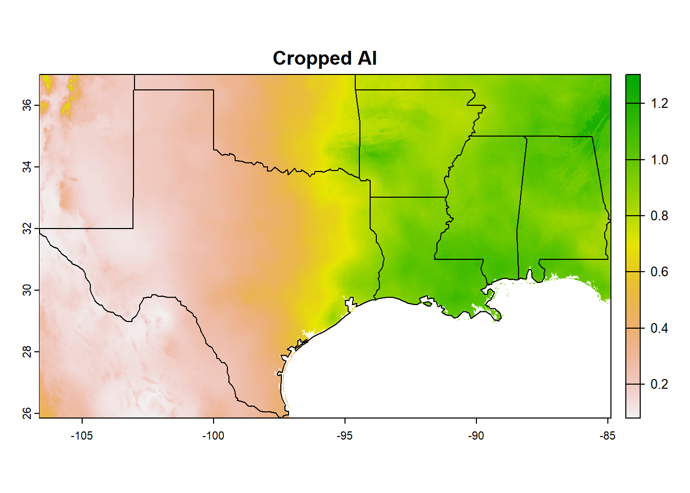
Cropping and masking operations are used to reduct the spatial extent of a raster/vector data. We will use US states shapefile from spData::us_states to select the polygons for Louisiana and adjoining states. The resource spData::us_states provides features for the Contiguous U.S. as simple feature, i.e., sf collection. We note that the state names in the us_states multipolygon are given in the field NAME, which we will use to subset the multipolygon to the specific states we are interested in. We will take “Louisiana”, “Texas”, “Mississippi”,“Alabama”, “Oklahoma”, “Arkansas” as examples.

library(spData)
library(sf)

AI=terra::rast("./SampleData-master/raster_files/P_over_ET0.tif") 

# Lets view the data
head(spData::us_states)

Simple feature collection with 6 features and 6 fields
Geometry type: MULTIPOLYGON
Dimension:     XY
Bounding box:  xmin: -114.8136 ymin: 24.55868 xmax: -71.78699 ymax: 42.04964
Geodetic CRS:  NAD83
  GEOID        NAME   REGION             AREA total_pop_10 total_pop_15
1    01     Alabama    South 133709.27 [km^2]      4712651      4830620
2    04     Arizona     West 295281.25 [km^2]      6246816      6641928
3    08    Colorado     West 269573.06 [km^2]      4887061      5278906
4    09 Connecticut Norteast  12976.59 [km^2]      3545837      3593222
5    12     Florida    South 151052.01 [km^2]     18511620     19645772
6    13     Georgia    South 152725.21 [km^2]      9468815     10006693
                        geometry
1 MULTIPOLYGON (((-88.20006 3...
2 MULTIPOLYGON (((-114.7196 3...
3 MULTIPOLYGON (((-109.0501 4...
4 MULTIPOLYGON (((-73.48731 4...
5 MULTIPOLYGON (((-81.81169 2...
6 MULTIPOLYGON (((-85.60516 3...

# From this we will subset the sf object for the selected states. We select forst column as we are only interested in a single attribute
US_shp=spData::us_states

# Subset selected states from the shapefile
south_sf=US_shp[US_shp$NAME %in% c("Louisiana", "Texas", "Mississippi","Alabama", "Oklahoma", "Arkansas"),]

# Convert the sf object to SpatRaster
south_vect=vect(south_sf)
plot(south_vect)

# Crop AIfine raster to south_vect extent 
AI_south=crop(AIfine, south_vect)
plot(AI_south, main="Cropped AI")
plot(south_vect, add=T)

# Mask AIfine raster to match south_vect spatial domain 
AI_south_msk=mask(AI_south, south_vect)   # Try: inverse=TRUE argument for fun
plot(AI_south_msk, main="Masked AI")
plot(south_vect, add=T)

Computing Counsel

1. For large rasters, it is computationally efficient to crop and/or mask rasters to the region of interest before the analysis.

2. crop first, and mask later, as masking is computationally expensive than cropping.

---

5.4 Raster RATification

In the AI plot above, we see the expected climate pattern for the terrestrial landmass. The eastern U.S. receives abundant precipitation, and have high aridity index values. In contrast, Southwestern US have hot and dry climate, and show low values of the aridity index. However, in common use, we are more familiar with the use of generalized climate categories, and not a numerical index. For example, its easier to understand, compare and contrast the difference between the climate of Arizona and Louisiana in terms of “arid” versus “humid”, than the respective AI values.

Such terms come from the United Nations Environment Program (UNEP, (Nash 1999)), that divides global climate in five discrete classes based on the aridity index as below:

Table 1: Aridity Index based climate classes given by UNEP

An attribute table can be added to a raster which serves as a look-up reference for the discrete classification of the continuous variable in the raster. This process of adding a Raster Attribute Table to a raster is called raster RAT-ification.

As an example, we will follow class breaks and names given in Table 1 to add a climate attribute to the AI raster. We will cut the pixel values of the AI raster into discrete classes and add the attribute table back to the original AI raster.

# Import AI raster and remove negative fill value
AI=terra::rast("./SampleData-master/raster_files/P_over_ET0.tif") 

# Breaks for each climate class from Table 1
class_brk= c(0, 0.03, 0.2, 0.5, 0.65, 10)                                
# Labels for each climate class from Table 1
class_names=c("Hyper arid", "Arid", "Semi arid", 
              "Sub humid", "Humid")   

# Divide the cell values in the AI raster into distinct levels
attributes=base::cut(values(AI), # Notice we apply cut on raster "values" 
                 breaks = class_brk,
                 labels =class_names )

# Add attributes to the SpatRaster as climate class
AI$climate = attributes
plot(AI$climate,  plg = list(loc = "bottomleft"))                    

5.5 Zonal Statistics

Zonal statistics refers to estimate statistical measures of the cell values of a raster within the zones of another dataset (raster/vector). In the subsequent examples, we will use the aridity index raster to create a polygon, demarcating the spatial boundaries of the discrete climate zones. We will then use these polygons to extract respective cell values and calculate zonal statistics for each climate.

5.5.1 Zonal Statistics with Polygons

5.5.1.1 Raster to Polygons

In the next example, we will convert the aridity raster into a polygon based on aridity classification using terra::as.polygons function.
We will use previously RATified the aridity index raster to generate polygons for the climate zones.

# Convert classified raster to shapefile
arid_poly=as.polygons(AI$climate)   # Convert SpatRaster to a spatial polygon 

# Notice the dimension (geometries, attributes) and values of the polygon. 
# Do the values match the classes you created?
print(arid_poly)

 class       : SpatVector 
 geometry    : polygons 
 dimensions  : 5, 1  (geometries, attributes)
 extent      : -124.7, -66.98333, 24.55833, 49.38333  (xmin, xmax, ymin, ymax)
 coord. ref. : lon/lat WGS 84 (EPSG:4326) 
 names       :    climate
 type        :      <chr>
 values      : Hyper arid
                     Arid
                Semi arid

# View polygon of the climate zones
library(mapview)
mapview(arid_poly)

# You can also crop SpatVectors
AI_poly_south=terra::crop(arid_poly, south_vect)
mapview(AI_poly_south)

5.5.1.2 Zonal Data Extraction and Statistics

Now we will use terra::extract function to extract the cell values of the soil moisture raster, sm, within each climate zone. We can then use tapply or the built-in fun option within terra::extract to calculate zonal statistics.

sm=terra::rast("./SampleData-master/raster_files/SMAP_SM.tif")

# Extract cell values for each climate class
sm_climate_df = terra::extract(sm,      # Raster to be summarized
                          arid_poly,    # Shapefile/ polygon to summarize the raster
                          na.rm=TRUE)   # Ignore NA values? yes! 
head(sm_climate_df)

  ID    SMAP_SM
1  1 0.06480984
2  1 0.08408742
3  1 0.05854325
4  1 0.05259301
5  1 0.04967655
6  1 0.04935537

# Calculate group-wise AI 
tapply(sm_climate_df$SMAP_SM,     # Column to be summarized
       sm_climate_df$ID,          # Grouping variable
       median,          # Function to use. User defined functions can be used too
       na.rm = TRUE)              # Ignore NA values? yes! 

         1          2          3          4          5 
0.07296192 0.06936086 0.14301015 0.21182603 0.32055609 

# OR: We can specify the "fun" argument within terra::extract function
sm_climate_median=terra::extract(sm,    # Raster to be summarized
                          arid_poly,    # Shapefile/ polygon to summarize the raster
                          fun=median,   # Statistic needed: median/mean/sum/min/max?
                          na.rm=TRUE)   # Ignore NA values? yes! 

# The climate-wise median values are extracted as a dataframe
head(sm_climate_median)

  ID    SMAP_SM
1  1 0.07296192
2  2 0.06936086
3  3 0.14301015
4  4 0.21182603
5  5 0.32055609

# Lets plot the climate-wise median of surface soil moisture
plot(sm_climate_median,     
     xaxt = "n",              # Disable x-tick labels
     xlab="Climate",          # X axis label
     ylab="Soil moisture",    # Y axis label
     type="b",                # line type
     col="blue",              # Line color
     main="Climate-wise median of surface soil moisture")
axis(1, at=1:5, labels=c("Hyper-arid", "Arid", "Semi-Arid","Sub-humid","Humid"))

Let us revisit our question:

How does the climate impact the spatial distribution of soil moisture?

Can we make a similar conclusion as before?

---

5.5.1.3 extract vs exact_extract

This is a good time to learn about another excellent function for raster cell extraction from the exactextractr package, exact_extract. This function is computationally faster and efficient than terra::extract, which will be evident when working with rasters of large size.

Remember:

1. exactextractr::exact_extract also outputs the fractional cell coverage of each pixel extracted. For some analysis (including ours), this information may not be needed.

2. exact_extract works on simple feature, sf, objects. So, we will use st_as_sf to convert SpatVector objects to sf.

library(exactextractr)
library(sf)

sm=terra::rast("./SampleData-master/raster_files/SMAP_SM.tif")

zonal_extract=exactextractr::exact_extract(sm,  # Raster to be summarized
                st_as_sf(arid_poly),    # Convert shapefile to sf (simple feature)
                force_df = TRUE,        # Output as a data.frame?
                include_xy = FALSE,     # Include cell lat-long in output?
                fun = NULL,             # Specify the function to apply for each feature extracted data
                progress = TRUE)        # Progressbar

  |                                                                            
  |                                                                      |   0%
  |                                                                            
  |==============                                                        |  20%
  |                                                                            
  |============================                                          |  40%
  |                                                                            
  |==========================================                            |  60%
  |                                                                            
  |========================================================              |  80%
  |                                                                            
  |======================================================================| 100%

zonal_data=sapply(zonal_extract,"[[",1)  # Select only cell values (first column within each element of the list)

# Generate boxplot for the zonal data
boxplot(zonal_data, 
        col=c("#800000", "#FF7C00","#87FF78","#008BFF","#00008F"), 
        names=c("Hyper arid", "Arid", "Semi arid","Sub humid", "Humid")  )

5.5.1.4 User-defined Functions for Zonal Statistics

Cell value extraction for each zone can help a user to carry a diverse set of analysis for each region using custom functions. Once the zonal cell values are extracted, vectorized application of user-defined function can be carried out on these datasets using lapply (list+apply) or purrr::map functions.

# Apply function on cell values for each zone

#~~ Using lapply
zonal_stat=lapply(zonal_data,median, na.rm=T)     # Returns a list of zonal stats

#~~ Using purrr::map
library(purrr)
zonal_stat=purrr::map(zonal_data,
                      ~ median(.x, na.rm=TRUE)) # Returns a list of zonal stats

#~~ Try user defined function
myfun=function (y){
  # User defined function for calculating median
  p=median(y, na.rm=TRUE)
  return(p)
  }    

#~ Implement function using lapply and map
#~~ Using lapply
zonal_stat=lapply(zonal_data,myfun)           # Returns a list of zonal median 

#~~ Using purrr::map
library(purrr)
zonal_stat=purrr::map(zonal_data,~ myfun(.x)) # Returns a list of zonal median 
zonal_stat=unlist(zonal_stat)                 # Unlist to return a vector 

head(zonal_stat) # Is this the same as the previous result?

[1] 0.06029825 0.07462480 0.12249910 0.18718112 0.31052290

5.5.2 Zonal Statistics with RATified Raster

Rasters with discrete data groups can also be used to summarize other rasters. Here, we will use the RATified aridity index raster to extract cell values corresponding to each climate zone.

zonal_data=list()                   # Create an empty list to store values
climate_num=as.numeric(AI$climate)  # Convert climate class to numerical values
climate_num=resample(climate_num,sm, method="near") # Resample to sm resolution 

# Extract pixel values within each climate zone
ZonalCells=function(x){
  zonalCells=na.omit(sm[climate_num==x])
  return(zonalCells)
} 
climate_zone_num=list(1,2,3,4,5)    # Store climate zone numbers as a list

# Apply function using lapply 
zonal_data=lapply(climate_zone_num,
                  ZonalCells)

# Calculate and store stats for each climate zone
#~~ Custom function for zonal median
zonalMean=function(x){
  zonalCells=na.omit(sm[climate_num==x])
  p=median(zonalCells, na.rm=TRUE)
  return(p)
} 
climate_zone_num=list(1,2,3,4,5)    # Store climate zone numbers as a list
zonal_stat_list=lapply(climate_zone_num,zonalMean)

# Equivalent to:
# zonal_stat_list=lapply(list(1,2,3,4,5),function(x) (median(sm[climate_num==x], na.rm=TRUE)))

# lapply returns a list, so we unlist the output to get an array
zonal_stat=unlist(zonal_stat_list)

plot(zonal_stat,     
     xaxt = "n",              # Disable x-tick labels
     xlab="Climate",          # X axis label
     ylab="Soil moisture",    # Y axis label
     type="b",                # line type
     col="blue",              # Line color
     main="Climate-wise median of surface soil moisture")
axis(1, at=1:5, labels=c("Hyper-arid", "Arid", "Semi-Arid","Sub-humid","Humid"))

---

Chen, Xi, and Murugesu Sivapalan. 2020. “Hydrological Basis of the Budyko Curve: Data-Guided Exploration of the Mediating Role of Soil Moisture.” Water Resources Research 56 (10): e2020WR028221.

Nash, David J. 1999. “World Atlas of Desertification.” The Geographical Journal 165: 325.

Schowengerdt, Robert A. 2007. “CHAPTER 7 - Correction and Calibration.” In Remote Sensing (Third Edition), edited by Robert A. Schowengerdt, Third Edition, 285–XXIII. Burlington: Academic Press. https://doi.org/https://doi.org/10.1016/B978-012369407-2/50010-3.

Zomer, Robert J, Jianchu Xu, and Antonio Trabucco. 2022. “Version 3 of the Global Aridity Index and Potential Evapotranspiration Database.” Scientific Data 9 (1): 409.